Film Study: All-22, Charting a Game, and Scoring Yourself

Watch it again the way a coach does, turn a game into rows you can count, and find out how good your Sunday calls really were.

Show the Python (shared drawing helpers for this chapter)
import os
import re
import tempfile
import textwrap
import logging

import numpy as np
import pandas as pd
import matplotlib.pyplot as plt
from matplotlib.patches import FancyBboxPatch, FancyArrowPatch, Rectangle, Circle, Patch
from matplotlib.lines import Line2D

from gridiron import Play, Player, offense, defense, routes as r, style, draw_marker, show_animation

logging.getLogger("matplotlib.font_manager").setLevel(logging.ERROR)
style.apply()
PDF = os.environ.get("RTG_FORMAT", "").lower() in ("pdf", "typst", "print")
LOOK = "#0f7a55"           # "look here" badges (a darker step of the aqua highlight)
AUTO_TINT = "#ecebe4"      # chart columns filled automatically from play-by-play
FILM_TINT = "#f6ecd2"      # chart columns that only your film can fill
LOG_TINT = "#dcefe6"       # your live log's columns


def pct(x, nd=0):
    """0.613 -> '61%'."""
    return f"{100 * x:.{nd}f}%"


def blank(ax):
    ax.set_axis_off()
    ax.grid(False)


def no_numbers(ax):
    """Remove the painted yard-line numbers (they sit where wide receivers and corners stand)."""
    for t in list(ax.texts):
        if t.get_alpha() == 0.55:
            t.remove()


def tag(fld, play, text, at, fs=7.0, ha="center", color=style.INK, bold=False, ec=style.BASELINE, z=21):
    """A boxed label at alignment coordinates (d, w), drawn above the players."""
    x, y = fld.xy(*play.to_abs(*at))
    fld.ax.text(x, y, text, ha=ha, va="center", fontsize=fs, color=color, zorder=z, linespacing=1.12,
                fontweight="bold" if bold else "normal",
                bbox=dict(boxstyle="round,pad=0.25", fc=style.SURFACE, ec=ec, lw=0.6))


def scorebug(fld, play, lines, at, fs=6.6, ha="left"):
    """A small dark scorebug box at (d, w)."""
    x, y = fld.xy(*play.to_abs(*at))
    fld.ax.text(x, y, "\n".join(lines), ha=ha, va="center", fontsize=fs, color="white", zorder=16,
                linespacing=1.25, fontweight="bold",
                bbox=dict(boxstyle="round,pad=0.35", fc="#2b2b2b", ec="none"))


# ------------------------------------------------------------------ print stand-ins for animations
def snapshot(play, t, ax, lateral, window, notes=(), trails=True):
    """Everyone where he is at time t, with faint trails of where he has been and the ball in flight."""
    pos = {k: play.position(k, t) for k in play.players}
    moved = [pl.moved(d=float(pos[k][0]), w=float(pos[k][1])) for k, pl in play.players.items()]
    q = Play([m for m in moved if m.side == "off"], [m for m in moved if m.side == "def"],
             los=play.los, ball_y=play.ball_y, to_go=play.to_go)
    q.highlights = dict(play.highlights)
    for n in notes:
        q.note(*n)
    fld = q.draw(ax=ax, lateral=lateral, window=window, title=False)
    no_numbers(fld.ax)
    P = lambda d, w: fld.xy(*play.to_abs(d, w))  # noqa: E731
    t0 = play._compile()[1]
    if trails:
        for k, pl in play.players.items():
            if pl.pos in ("LT", "LG", "C", "RG", "RT"):
                continue
            pts = np.array([play.position(k, tt) for tt in np.linspace(t0, t, 40)])
            if np.ptp(pts[:, 0]) + np.ptp(pts[:, 1]) < 0.4:
                continue
            xs, ys = P(pts[:, 0], pts[:, 1])
            col = style.OFFENSE if pl.side == "off" else style.DEFENSE
            ls = "-" if pl.side == "off" else (0, (3, 2))
            ax.plot(xs, ys, color=col, lw=1.0, alpha=0.5, ls=ls, zorder=3)
    if t > 0:
        for who, tgt in play.reads:                               # the quarterback's eyes
            (x0, y0), (x1, y1) = P(*play.position(who, t)), P(*play.position(tgt, t))
            ax.plot([float(x0), float(x1)], [float(y0), float(y1)], color=style.THIRD, lw=1.2, ls=(0, (4, 2)),
                    zorder=4)
    return fld


def strip(play, times, labels, lateral, window, ncols=2, width_in=6.5):
    """The print version of an animation: one panel per moment, each titled with what to see."""
    n = len(times)
    nrows = int(np.ceil(n / ncols))
    pw = width_in / ncols
    h = nrows * (pw * (window[1] - window[0]) / abs(lateral[1] - lateral[0]) + 0.36)
    fig, axes = plt.subplots(nrows, ncols, figsize=(width_in, h), squeeze=False)
    for ax in axes.flat[n:]:
        ax.axis("off")
    for ax, t, lab in zip(axes.flat, times, labels):
        snapshot(play, t, ax, lateral, window)
        ax.set_title(lab, fontsize=8.2, color=style.INK, loc="left")
    fig.tight_layout(h_pad=0.5, w_pad=0.4)
    return fig


def animate_or_strip(play, times, labels, lateral, window):
    """Video on the web, a titled frame strip in print."""
    if PDF:
        strip(play, times, labels, lateral, window)
        plt.show()
    else:
        show_animation(play, times=times)


def wash(fld, play, t, keys, reads=False, alpha=0.66, half=()):
    """Fade the whole picture, then redraw only `keys` (with their trails) on top: one pass of the film.
    Players in `half` are redrawn at half strength, as context for the group being watched."""
    ax = fld.ax
    (x0, x1), (y0, y1) = ax.get_xlim(), ax.get_ylim()
    ax.add_patch(Rectangle((min(x0, x1), min(y0, y1)), abs(x1 - x0), abs(y1 - y0), fc=style.SURFACE, ec="none",
                           alpha=alpha, zorder=12))
    ppy = fld.pts_per_yard()
    P = lambda d, w: fld.xy(*play.to_abs(d, w))  # noqa: E731
    t0 = play._compile()[1]
    for k in list(half) + list(keys):
        pl = play.players[k]
        a_ = 0.5 if k in half else 1.0
        pts = np.array([play.position(k, tt) for tt in np.linspace(t0, t, 50)])
        if np.ptp(pts[:, 0]) + np.ptp(pts[:, 1]) > 0.4:
            xs, ys = P(pts[:, 0], pts[:, 1])
            col = style.OFFENSE if pl.side == "off" else style.DEFENSE
            ax.plot(xs, ys, color=col, lw=1.4, alpha=a_, ls="-" if pl.side == "off" else (0, (3, 2)), zorder=13)
        x, y = P(*play.position(k, t))
        for a in draw_marker(ax, float(x), float(y), pl.side, pl.label, ppy, ring=play.highlights.get(k)):
            a.set_zorder(a.get_zorder() + 10)
            if a_ < 1:
                a.set_alpha(a_)
    if reads:
        for who, tgt in play.reads:
            (xa, ya), (xb, yb) = P(*play.position(who, t)), P(*play.position(tgt, t))
            ax.plot([float(xa), float(xb)], [float(ya), float(yb)], color=style.THIRD, lw=1.4, ls=(0, (4, 2)),
                    zorder=13)


def protect(p, linemen=("LT", "LG", "C", "RG", "RT")):
    """Linemen set back into pass protection."""
    for k in linemen:
        p.block(k, pts=[(-1.2, 0.0)])


from gridiron.play import _interp  # noqa: E402  (keyframe interpolation, used by the trail-technique play below)


class TrailPlay(Play):
    """A Play whose man defenders play trail technique: from their alignment at the snap they settle, within
    about a second, a yard behind and a yard inside their receiver ("on his inside hip, underneath").
    gridiron's own p.man() closes the cushion to almost nothing, which draws the defender on top of the
    receiver and hides him; this keeps both visible, and it's the technique 2-Man actually asks for."""

    def __init__(self, *a, **k):
        super().__init__(*a, **k)
        self.trail = {}

    def trail_man(self, key, target, behind=1.0, inside=1.1, lag=0.15, settle=1.0):
        self.trail[key] = (target, behind, inside, lag, settle)
        self._compiled = None
        return self

    def _compile(self):
        if self._compiled is not None:
            return self._compiled
        kf, t_start, t_end = super()._compile()
        for key, (tgt, behind, inside, lag, settle) in self.trail.items():
            own, rec = kf[key], kf[tgt]
            s0, r0 = _interp(own, 0.0), _interp(rec, 0.0)
            off0 = s0 - r0
            want = np.array([-behind, -np.sign(r0[1]) * inside])          # behind him, toward the ball
            rows = [row for row in own if row[0] < 0]
            for t in np.linspace(0.0, t_end + 0.6, 70):
                f = np.clip(t / settle, 0, 1)
                f = f * f * (3 - 2 * f)                                     # ease in, ease out
                rows.append((t, *(_interp(rec, max(t - lag, 0.0)) + off0 * (1 - f) + want * f)))
            kf[key] = np.array(rows, dtype=float)
        self._compiled = (kf, t_start, t_end)
        return self._compiled
Show the Python (data: nflverse play-by-play, FTN charting and participation, 2024–2025)
from gridiron.data import pbp, nfl

PCOLS = ["season_type", "game_id", "play_id", "posteam", "defteam", "play_type", "down", "ydstogo", "yardline_100",
         "yrdln", "pass", "qb_dropback", "xpass", "week", "qtr", "time", "fixed_drive", "fixed_drive_result",
         "yards_gained", "epa", "success", "sack", "interception", "fumble_lost", "touchdown", "pass_location",
         "run_location", "score_differential", "desc", "rusher_player_name", "receiver_player_name"]
FTN_COLS = ["game_id", "play_id", "starting_hash", "qb_location", "n_offense_backfield", "is_motion", "is_no_huddle",
            "is_play_action", "is_screen_pass", "is_rpo", "n_pass_rushers", "n_blitzers"]
PART_COLS = ["game_id", "play_id", "offense_personnel", "defense_personnel", "defenders_in_box",
             "defense_coverage_type", "defense_man_zone_type", "was_pressure", "time_to_throw"]


def load_season(season):
    """Runs and dropbacks, with FTN charting and participation attached."""
    d = pbp([season], columns=PCOLS)
    d = d[d.play_type.isin(["pass", "run"]) & d.down.notna()].copy()
    d["play_id"] = d.play_id.astype(float)
    f = nfl().load_ftn_charting([season]).to_pandas()
    f = f.rename(columns={"nflverse_game_id": "game_id", "nflverse_play_id": "play_id"})
    f["play_id"] = f.play_id.astype(float)
    p = nfl().load_participation([season]).to_pandas().rename(columns={"nflverse_game_id": "game_id"})
    p["play_id"] = p.play_id.astype(float)
    return (d.merge(f[FTN_COLS], on=["game_id", "play_id"], how="left")
             .merge(p[PART_COLS], on=["game_id", "play_id"], how="left"))


def count_pos(s, keys):
    if not isinstance(s, str):
        return np.nan
    c = {k: int(v) for v, k in re.findall(r"(\d+) ([A-Z]+)", s)}
    return sum(c.get(k, 0) for k in keys)


def pers_code(s):
    """FTN-era personnel string ('1 C, 2 G, 1 QB, 1 RB, 2 T, 1 TE, 3 WR') -> '11'."""
    if not isinstance(s, str):
        return "?"
    c = {k: int(v) for v, k in re.findall(r"(\d+) ([A-Z]+)", s)}
    return f"{c.get('RB', 0) + c.get('FB', 0)}{c.get('TE', 0)}"


COV = {"COVER_0": "C0", "COVER_1": "C1", "COVER_2": "C2", "2_MAN": "2M", "COVER_3": "C3", "COVER_4": "C4",
       "COVER_6": "C6", "COVER_9": "C9", "COMBO": "CMB", "BLOWN": "BLN", "PREVENT": "PRV"}
TWO_HIGH = {"C2", "2M", "C4", "C6"}
ONE_HIGH = {"C0", "C1", "C3", "C9"}          # C0 has nobody deep; "not two-high" for the shell call


def chart_codes(d):
    """The public charting, written in the chart sheet's short codes."""
    d = d.copy()
    d["pers"] = d.offense_personnel.map(pers_code)
    nb = d.n_offense_backfield
    d["align"] = d.qb_location.fillna("?") + nb.map(lambda v: "?" if pd.isna(v) else str(int(min(v, 2))))
    d["mot"] = np.where(d.is_motion.fillna(False).astype(bool), "M", "–")
    d["ndb"] = d.defense_personnel.map(lambda s: count_pos(s, ("CB", "FS", "SS", "S", "DB")))
    d["dpers"] = d.ndb.map(lambda v: {4: "base", 5: "nickel", 6: "dime", 7: "quarter"}.get(int(v), "?")
                           if pd.notna(v) else "?")
    d["box"] = d.defenders_in_box.map(lambda v: "?" if pd.isna(v) else str(int(v)))
    d["cv"] = d.defense_coverage_type.map(COV)
    d["rush"] = d.n_pass_rushers
    kind = np.where(d.qb_dropback == 1, "P", "R")
    kind = np.where(d.is_play_action.fillna(False).astype(bool) & (kind == "P"), "PA", kind)
    kind = np.where(d.is_screen_pass.fillna(False).astype(bool), "SCR", kind)
    d["kind"] = kind
    d["is_pass"] = (d.qb_dropback == 1).astype(int)

    def res(row):
        if row.sack == 1:
            return "sk FUM" if row.fumble_lost == 1 else f"sk {int(row.yards_gained):+d}".replace("-", "−")
        if row.interception == 1:
            return "INT"
        if row.fumble_lost == 1:
            return "FUM"
        if row.touchdown == 1:
            return "TD"
        return f"{int(row.yards_gained):+d}".replace("-", "−")
    d["res"] = d.apply(res, axis=1)
    d["hash"] = d.starting_hash.where(d.starting_hash.isin(["L", "M", "R"]), "?")   # FTN writes 0 when unknown
    return d


S24 = load_season(2024)
S25 = load_season(2025)

# ------------------------------------------------------------------ Super Bowl LX, both offenses
SB_ID = "2025_22_SEA_NE"
SB = chart_codes(S25[S25.game_id == SB_ID]).sort_values("play_id").reset_index(drop=True)
NE = SB[SB.posteam == "NE"]
SEA = SB[SB.posteam == "SEA"]
NE_DB = NE[NE.qb_dropback == 1]
NE_LAB = NE_DB[NE_DB.cv.isin(TWO_HIGH | ONE_HIGH)]
SBX = dict(
    ne_snaps=len(NE), ne_db=len(NE_DB), ne_pass=float(NE.is_pass.mean()),
    four=int((NE_DB.rush == 4).sum()), five=int((NE_DB.rush >= 5).sum()),
    sacks=int(NE.sack.sum()), sacks4=int(((NE.sack == 1) & (NE.rush == 4)).sum()),
    press=float(NE_DB.was_pressure.fillna(False).astype(float).mean()),
    two=float(NE_LAB.cv.isin(TWO_HIGH).mean()), n_lab=len(NE_LAB),
    man=float((NE_DB.defense_man_zone_type == "MAN_COVERAGE").sum()
              / NE_DB.defense_man_zone_type.isin(["MAN_COVERAGE", "ZONE_COVERAGE"]).sum()),
    sea_snaps=len(SEA), sea_run=float(1 - SEA.is_pass.mean()), sea_uc=float((SEA.qb_location == "U").mean()),
    walker_n=int((SEA.rusher_player_name == "K.Walker").sum()),
    walker_y=int(SEA.loc[SEA.rusher_player_name == "K.Walker", "yards_gained"].sum()),
    ne_succ=float(NE.success.mean()), sea_succ=float(SEA.success.mean()),
)

_R25 = S25[S25.season_type == "REG"]
SBX["ne_reg_pass"] = float(_R25.loc[_R25.posteam == "NE", "qb_dropback"].mean())
SBX["sea_reg_run"] = float(1 - _R25.loc[_R25.posteam == "SEA", "qb_dropback"].mean())

# Seattle's defense against dropbacks in the 2025 regular season, and the league's
REG = S25[(S25.season_type == "REG") & (S25.qb_dropback == 1)].copy()
REG["c"] = REG.defense_coverage_type.map(COV)
REG_LAB = REG[REG.c.isin(TWO_HIGH | ONE_HIGH)]
SEA_REG = REG_LAB[REG_LAB.defteam == "SEA"]
SEASON = dict(sea_two=float(SEA_REG.c.isin(TWO_HIGH).mean()), lg_two=float(REG_LAB.c.isin(TWO_HIGH).mean()),
              sea_four=float((REG[(REG.defteam == "SEA") & (REG.n_pass_rushers > 0)].n_pass_rushers == 4).mean()),
              lg_four=float((REG[REG.n_pass_rushers > 0].n_pass_rushers == 4).mean()),
              sea_press=float(REG.loc[REG.defteam == "SEA", "was_pressure"].fillna(False).astype(float).mean()),
              lg_press=float(REG.was_pressure.fillna(False).astype(float).mean()))


def sea_two_rate(down):
    """Seattle's 2025 regular-season two-high rate on dropbacks, by down (1st, 2nd, 3rd/4th)."""
    dd = SEA_REG.down.clip(upper=3)
    return float(SEA_REG.loc[dd == min(down, 3), "c"].isin(TWO_HIGH).mean())


# The strip-sack: third-and-6, end of the third quarter
SS_ROW = NE[(NE.qtr == 3) & (NE.sack == 1) & (NE.fumble_lost == 1)].iloc[0]

# ------------------------------------------------------------------ the pre-snap model (situation + formation)
def feats(d):
    xp = np.clip(d.xpass.astype(float), 1e-3, 1 - 1e-3)
    nb = d.n_offense_backfield.fillna(1)
    return np.column_stack([np.ones(len(d)), np.log(xp / (1 - xp)), d.qb_location == "S", d.qb_location == "P",
                            nb == 0, nb >= 2]).astype(float)


def fit(X, y, lam=1.0, iters=30):
    """Ridge-penalised logistic regression by Newton's method (numpy only)."""
    w = np.zeros(X.shape[1])
    for _ in range(iters):
        p = 1 / (1 + np.exp(-X @ w))
        H = X.T @ (X * (p * (1 - p))[:, None]) + lam * np.eye(X.shape[1])
        w -= np.linalg.solve(H, X.T @ (p - y) + lam * w)
    return w


TR = S24[(S24.season_type == "REG") & S24.xpass.notna()]
W_INFO = fit(feats(TR), TR["pass"].values.astype(float))


def p_info(d):
    return 1 / (1 + np.exp(-feats(d) @ W_INFO))


def conf_of(p, cap=0.9):
    return float(np.clip(np.round(max(p, 1 - p) * 20) / 20, 0.5, cap))


SB["p_rule"] = p_info(SB)
SB["call"] = np.where(SB.p_rule >= 0.5, "P", "R")
SB["conf"] = SB.p_rule.map(conf_of)

# ------------------------------------------------------------------ a simulated reader: every Panthers snap of 2025
CAR = S25[(S25.posteam == "CAR") & S25.xpass.notna()].sort_values(["week", "play_id"]).reset_index(drop=True)
CAR["p_info"] = p_info(CAR)
GAMES = list(dict.fromkeys(CAR.game_id))
CAR["g"] = CAR.game_id.map({g: i for i, g in enumerate(GAMES)})
N_GAMES = len(GAMES)
LG = np.log(CAR.p_info / (1 - CAR.p_info)).values
Y = CAR["pass"].values.astype(int)


def simulate(k0, k1, s0, s1, cap0, cap1, seed):
    """A reader who sees what the model sees, through noise, and over- or under-states it.
    k > 1 overstates, k < 1 understates; both settle over the season from (k0, s0, cap0) to (k1, s1, cap1)."""
    rng = np.random.default_rng(seed)
    frac = (CAR.g / (N_GAMES - 1)).values
    k, sd = k0 + (k1 - k0) * frac, s0 + (s1 - s0) * frac
    cap = np.where(frac < 0.45, cap0, cap1)
    pr = 1 / (1 + np.exp(-(k * LG + rng.normal(0, 1, len(CAR)) * sd)))
    conf = np.clip(np.round(np.maximum(pr, 1 - pr) * 20) / 20, 0.5, cap)
    return np.where(pr >= 0.5, "P", "R"), conf


ME_CALL, ME_CONF = simulate(1.5, 0.95, 0.6, 0.4, 0.95, 0.90, seed=15)
A_CALL, A_CONF = simulate(2.2, 2.2, 0.3, 0.3, 0.99, 0.99, seed=7)
B_CALL, B_CONF = simulate(0.35, 0.35, 0.1, 0.1, 0.85, 0.85, seed=7)


LOGDF = pd.DataFrame({
    "game": CAR.g + 1, "week": CAR.week.astype(int), "opp": CAR.defteam, "down": CAR.down.astype(int),
    "togo": CAR.ydstogo.astype(int), "align": CAR.qb_location.fillna("?") + CAR.n_offense_backfield.map(
        lambda v: "?" if pd.isna(v) else str(int(min(v, 2)))),
    "call": ME_CALL, "conf": ME_CONF,
    "clue": np.where(np.abs(CAR.p_info - CAR.xpass) > 0.10, "align", "sit"),
    "result": np.where(Y == 1, "P", "R")})
HIT = (LOGDF.call == LOGDF.result).values.astype(float)


def brier_of(conf, hit):
    return float(np.mean((np.asarray(conf) - np.asarray(hit)) ** 2))


BASE_P = float(Y.mean())
REF = dict(half=0.25, base=BASE_P * (1 - BASE_P), xpass=float(np.mean((CAR.xpass.values - Y) ** 2)),
           info=float(np.mean((CAR.p_info.values - Y) ** 2)), me=brier_of(ME_CONF, HIT))
FIRST = (CAR.g < 8).values
ME = dict(n=len(CAR), acc=float(HIT.mean()), conf=float(ME_CONF.mean()),
          b1=brier_of(ME_CONF[FIRST], HIT[FIRST]), b2=brier_of(ME_CONF[~FIRST], HIT[~FIRST]),
          a1=float(HIT[FIRST].mean()), a2=float(HIT[~FIRST].mean()),
          c1=float(ME_CONF[FIRST].mean()), c2=float(ME_CONF[~FIRST].mean()),
          xpass_acc=float(((CAR.xpass >= 0.5).astype(int) == Y).mean()),
          info_acc=float(((CAR.p_info >= 0.5).astype(int) == Y).mean()))
DD_RUN = ((CAR.ydstogo <= 3) & (CAR.down != 3)) | ((CAR.down == 1) & (CAR.ydstogo <= 6))
ME["dd_acc"] = float((np.where(DD_RUN, 0, 1) == Y).mean())
_AL = (LOGDF.clue == "align").values
ME["align_me"] = float(HIT[_AL].mean())
ME["align_x"] = float(((CAR.xpass.values[_AL] >= 0.5).astype(int) == Y[_AL]).mean())
ME["always"] = BASE_P


def top_band(conf, hit, lo):
    m = np.asarray(conf) >= lo
    return float(np.asarray(hit)[m].mean()), int(m.sum())


ME["top1"], ME["n_top1"] = top_band(ME_CONF[FIRST], HIT[FIRST], 0.9)
ME["top2"], ME["n_top2"] = top_band(ME_CONF[~FIRST], HIT[~FIRST], 0.9)
ME["mid1"], ME["n_mid1"] = (lambda m: (float(HIT[FIRST][m].mean()), int(m.sum())))(
    (ME_CONF[FIRST] >= 0.7) & (ME_CONF[FIRST] < 0.8))

# Readers A and B for the drill
HIT_A = ((A_CALL == "P") == (Y == 1)).astype(float)
HIT_B = ((B_CALL == "P") == (Y == 1)).astype(float)


def recalibrated(conf, hit):
    """Brier score if every stated value were replaced by its own hit rate (perfect calibration, same calls)."""
    t = pd.DataFrame({"c": conf, "h": hit})
    return brier_of(t.groupby("c").h.transform("mean"), t.h)


AB = dict(a_acc=float(HIT_A.mean()), b_acc=float(HIT_B.mean()), a_b=brier_of(A_CONF, HIT_A),
          b_b=brier_of(B_CONF, HIT_B), a_conf=float(A_CONF.mean()), b_conf=float(B_CONF.mean()),
          a_fix=recalibrated(A_CONF, HIT_A), b_fix=recalibrated(B_CONF, HIT_B),
          a_90=top_band(A_CONF, HIT_A, 0.9), b_top=float(B_CONF.max()))


def murphy(f, o):
    """Brier = reliability − resolution + uncertainty (Murphy 1973), grouping by the distinct forecast values."""
    t = pd.DataFrame({"f": f, "o": o})
    g = t.groupby("f").o.agg(["size", "mean"])
    ob = t.o.mean()
    rel = float((g["size"] * (g.index - g["mean"]) ** 2).sum() / len(t))
    res = float((g["size"] * (g["mean"] - ob) ** 2).sum() / len(t))
    return rel, res, float(ob * (1 - ob))


F_PASS = np.where(ME_CALL == "P", ME_CONF, 1 - ME_CONF)          # the same calls, as a chance of a pass
MUR1 = murphy(F_PASS[FIRST], Y[FIRST])
MUR2 = murphy(F_PASS[~FIRST], Y[~FIRST])

# the season in four stretches (the same split the scoring code prints)
_PART = pd.cut(LOGDF.game, [0, 4, 8, 13, 18], labels=False)
QTR = [brier_of(ME_CONF[_PART == i], HIT[_PART == i]) for i in range(4)]
QTR_ACC = [float(HIT[_PART == i].mean()) for i in range(4)]
QTR_CONF = [float(ME_CONF[_PART == i].mean()) for i in range(4)]


def group_cost(c, h):
    """Expected Brier score per call for a group stated at c that came true a share h of the time."""
    return h * (1 - c) ** 2 + (1 - h) * c ** 2


_A90 = A_CONF >= 0.9
AB["a90_c"], AB["a90_share"] = float(A_CONF[_A90].mean()), float(_A90.mean())
AB["a90_cost"] = group_cost(AB["a90_c"], AB["a_90"][0])
AB["a90_fixcost"] = group_cost(AB["a_90"][0], AB["a_90"][0])
_B_LO = B_CONF <= 0.65
AB["b_lo_c"], AB["b_lo_h"], AB["b_lo_share"] = (float(B_CONF[_B_LO].mean()), float(HIT_B[_B_LO].mean()),
                                                float(_B_LO.mean()))
AB["b_lo_cost"] = group_cost(AB["b_lo_c"], AB["b_lo_h"])

# Seattle's 2025 two-high rate by down, as printed on the scouting card in the second-layer code below
CARD = {d_: round(sea_two_rate(d_), 2) for d_ in (1, 2, 3)}
Super Bowl LX, February 8, 2026. Seattle sacked Drake Maye 6 times, and every one of them looked the same on television: a pass rusher, a quarterback going down, a replay of the rusher’s celebration. What the broadcast never showed was why. On 5 of those 6 sacks, the charting says, Seattle rushed only four players, which means New England had at least five blockers for four rushers and seven Seahawks were covering. So was it the rush? The coverage? A quarterback holding the ball? A play call that sent everyone deep on the wrong down? You can’t answer that from the couch on Sunday. You can answer it on Monday, with the coaches’ film, a pause button and a routine, and that’s where this chapter starts. It ends with the other thing Monday is for: taking the season of predictions you’ve been logging since Part 1 and finding out, with a number, how good they were.

You’ll be able to…

NoteYou’ll need

This is the last chapter, and it leans on three earlier ones more than the rest:

What Sunday can’t tell you

Live watching, done well, is prediction. You read the situation and the formation, make a call with a number on it, and the snap tells you whether the call was right. But the snap only answers the first layer. It tells you pass; it doesn’t tell you whether the coverage you called was the coverage that was played, because the camera was on the quarterback when the safeties turned. It tells you sack; it doesn’t tell you whose fault the sack was. It tells you seven-yard run; it doesn’t tell you whether the run went where it was designed to go or bounced somewhere else because a block failed. And after a season of logging, a nagging question: you’ve been writing “70%” next to calls for months. Do your 70% calls come true seven times in ten?

Those are three different gaps, and this chapter closes each with its own tool:

  1. The film answers what happened, for every player, on every snap. It’s the only source that shows all 22 at once for the whole play.
  2. The chart turns what happened into rows: one per snap, the same fields every time, so a game can be counted instead of remembered. It is also the answer key for your log’s second layer.
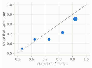
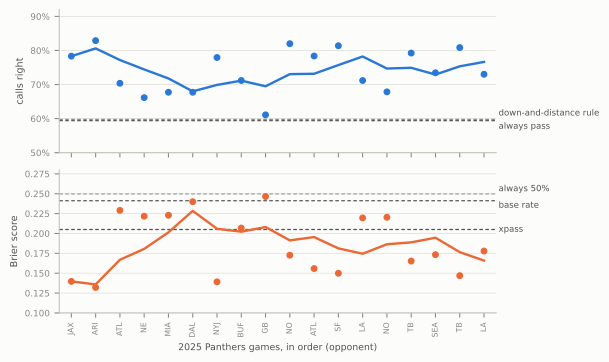
  3. The score turns your log into a number that rewards both being right and being honest about how sure you were, and a plot that tells you which way to adjust.

Coaches have done the first two for as long as there has been film. In an NFL building, Monday morning belongs to the last game: every player graded on every snap, the staff deciding what to fix, and the quality control coaches’ tags on every snap feeding the reports the coordinators read (The Game Plan: A Week Inside an NFL Building). The third is borrowed from weather forecasters, who have been scored this way since 1950. You’ll do a fan’s version of all three, with free data, an affordable film subscription and a few dozen lines of Python.

ImportantWhy it exists: watching the same play four times

Why not just watch the replay carefully once? Because attention is narrower than it feels. In a famous experiment, viewers asked to count basketball passes in a short video missed a person in a gorilla suit walking through the middle of the scene; about half of them never saw it.1 Football film is that experiment on every snap: watch the quarterback and you won’t see the safety rotate; watch the safety and you won’t see which lineman lost. Coaches solved this long ago by dividing the film: the offensive line coach watches the line, the secondary coach the secondary. A fan has no staff, so you divide the film by time instead, watching the same snap several times, a different group each time.

What it gives up: time. Four passes on every snap of a game is hours of work, which is why the protocol below comes with a short version.

Getting the film

You met coaches film in How to Watch a Broadcast: every snap shown twice, once from the high wide sideline angle that keeps all 22 players in frame, and once from a high camera behind the end zone. Fans have been able to buy it since 2012. Today it comes with NFL+ Premium, the league’s own subscription: it was part of Premium for the 2026 season, and when the league described the package in 2024 its archive went back to the 2022 season.2 It isn’t posted the moment the game ends: the league’s help pages say to expect it 24 to 36 hours after the final whistle, so a Sunday game is ready by Monday night or Tuesday. Packages and prices change often, so check what’s included before you pay.

If you don’t have it, you can still do a lot with what’s free. The broadcast’s own replays include the skycam and end-zone angles on many snaps. Teams post highlight clips, and several film-breakdown writers post All-22 clips of the plays they analyse (there’s a list at the end of the chapter). None of it is every snap from every angle, which is what charting a whole game needs, but it’s plenty for studying the snaps that mattered. (Which chart columns the broadcast alone can fill is in the codebook below.)

Setting up. Three things, side by side if you have the screen for it:

  • The film, in a player that can pause cleanly on a single frame, step a frame at a time, and slow down to half speed. Most of what you’ll do is pause on the snap, play a second and a half, and go back. If the subscription’s own player won’t step frames on your device, try it on a computer’s browser before you give up on it.
  • The chart, a spreadsheet with one row per snap (the template is below), already filled with everything the play-by-play knows, so you only type what the film adds.
  • Your live log, the sheet you kept on Sunday. You’ll check it against the film, but you won’t change it: it’s a record of what you knew before the snap, and correcting it after watching the film would make your score meaningless. Film notes go in their own column, marked as written after the fact.

Keeping the three lined up. Coaches film has no scorebug, so it can’t tell you which snap you’re on; the play-by-play can. Every row carries the quarter, the clock at the snap, the down and distance and the ball’s spot (qtr, time, down, ydstogo and yrdln in nflverse), and the film shows the snaps in the order they happened. Number the snaps in the chart, keep a finger on the down and distance and the yard line (both visible on the field), and the film, the chart and your log stay on the same row. Your log already has the quarter and clock from Sunday, which is how the two get joined later.

Timing a snap. Several passes below ask you to count seconds from the snap. A phone stopwatch started on the snap is good to a few tenths, which is enough to tell 2 seconds from 3.5. For better, step frames: video usually runs at 30 or 60 frames a second, so at 30, two and a half seconds is 75 frames.

Knowing who’s who. Jersey numbers are small in the wide shot. Keep both teams’ rosters open, identify players by where they line up first (the left tackle is the left tackle whatever his number), and confirm a number on the end-zone angle when it matters.

The four-pass film protocol

Here is the routine. It’s the course’s film-study protocol: a fixed way to study each snap on film, the same way every time. You freeze the picture at the snap and check your pre-snap read; then you watch the play four times, once for each group (the line, the quarterback, the coverage, the receivers and backs); then you write one line saying why the play worked or failed. Before any of that, watch the snap once at full speed, to see the play whole and where the ball went.

Each step uses the angle that shows its group best. The All-22 is the only one with every player in frame, so it’s the angle for the freeze, the coverage and the routes. The end-zone camera looks straight down the line, so it’s the angle for the blocks and for the quarterback’s feet and eyes.

Show the Python
items = [
    ("0", "Freeze at the snap",
     "One look at full speed, then pause on the snap. Check the log's pre-snap columns: personnel, formation and "
     "strength, motion and the defense's answer, box, shell, leverage. Write what you missed live.", "All-22",
     "Your read was made here; grade it before you know the result"),
    ("1", "The line (and the front)",
     "First step: forward (run) or back (pass). Run: zone or gap, who pulled, who was left unblocked on purpose, "
     "where the hole opened. Pass: blockers against rushers, the slide, who came free, and when.", "End zone",
     "The line decides how much time everyone else gets"),
    ("2", "The quarterback",
     "Drop and launch point; where his eyes went first; on time or late (count it); the throw he chose against "
     "the one that was there; what pressure did to him. Runs: the mesh and any read.", "End zone,\nthen All-22",
     "Judge what he did with the time pass 1 measured"),
    ("3", "The coverage",
     "Safeties first: their first step, where they finished (middle open or closed). Corners: bail, squat or "
     "trail. Who traveled with motion, who blitzed, who replaced him. Name it, with a confidence.", "All-22",
     "The hardest read; by now you know where the ball went"),
    ("4", "The skill players",
     "The routes as one concept; who was open at the moment the quarterback looked; separation and yards after "
     "the catch. Runs: the back's aim, his cut, yards after contact; blocks by receivers and tight ends.", "All-22",
     "Routes only make sense against the coverage"),
    ("✓", "The 'because' line",
     "One line: why it worked or failed, and whose play it was (either side's call, the line, the quarterback, the "
     "coverage, the skill players). Then fill in the chart row.", "",
     "A snap you can't explain in one line needs another pass"),
]
rows = []
for num, head, body, view, why in items:
    lines_ = textwrap.wrap(body, 56)
    why_ = textwrap.wrap(why, 27)
    rows.append((num, head, lines_, view, why_, max(len(lines_) + 1, len(why_), 2)))
H = sum(r_[5] for r_ in rows) + 0.35 * len(rows) + 3.4
fig, ax = plt.subplots(figsize=(6.5, 0.19 * H))
fig.subplots_adjust(left=0, right=1, top=1, bottom=0)
ax.set_xlim(0, 100)
ax.set_ylim(0, H)
ax.axis("off")
ax.add_patch(FancyBboxPatch((0.8, 0.3), 98.4, H - 0.6, boxstyle="round,pad=0.2,rounding_size=0.8",
                            fc=style.SURFACE, ec=style.BASELINE, lw=1.2))
ax.text(3, H - 1.25, "The four-pass film protocol", fontsize=11.5, fontweight="bold", color=style.INK, va="center")
ax.text(97, H - 1.25, "one snap, about two minutes", fontsize=7.6, color=style.INK_2, ha="right", va="center")
ax.text(9.0, H - 2.55, "WATCH FOR", fontsize=6.6, fontweight="bold", color=style.INK_2, va="center")
ax.text(60.5, H - 2.55, "ANGLE", fontsize=6.6, fontweight="bold", color=style.INK_2, va="center")
ax.text(72.0, H - 2.55, "WHY HERE", fontsize=6.6, fontweight="bold", color=style.INK_2, va="center")
y = H - 3.6
for k, (num, head, lines_, view, why_, h) in enumerate(rows):
    top, bottom = y + 0.55, y - (h - 1) - 0.45
    fc = LOG_TINT if num in ("0", "✓") else "#eef3fb"
    ax.add_patch(FancyBboxPatch((2.2, bottom), 95.6, top - bottom, boxstyle="round,pad=0.05,rounding_size=0.4",
                                fc=fc, ec="none"))
    ax.scatter([5.3], [y - 0.05], s=150, color=LOOK, edgecolor="white", linewidth=0.8, zorder=5)
    ax.text(5.3, y - 0.05, num, ha="center", va="center", fontsize=7.4, color="white", fontweight="bold", zorder=6)
    ax.text(9.0, y, head, fontsize=8.2, fontweight="bold", color=style.INK, va="center")
    for j, ln in enumerate(lines_):
        ax.text(9.0, y - 1 - j, ln, fontsize=7.0, color=style.INK, va="center")
    for j, ln in enumerate(view.split("\n")):
        ax.text(60.5, y - j, ln, fontsize=6.9, color=style.OFFENSE_DARK, va="center", fontweight="bold")
    for j, ln in enumerate(why_):
        ax.text(72.0, y - j, ln, fontsize=6.7, color=style.INK_2, va="center", style="italic")
    y -= h + 0.35
plt.show()
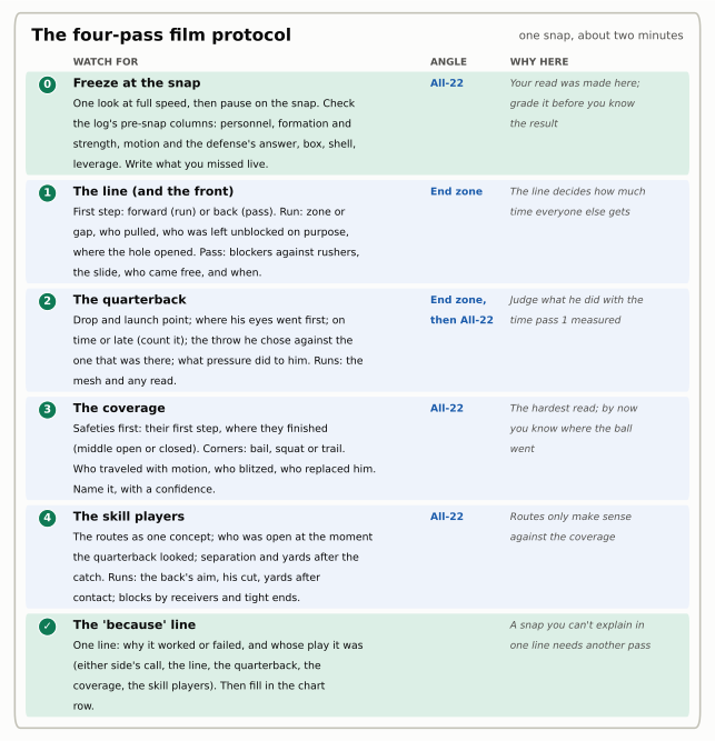
Figure 75.1: The protocol on one card, to keep beside the film. The middle column is the angle of the coaches film to use for each step; the right-hand column is why the step sits where it does: the order runs from what sets the play’s clock (the line) to what uses it (the routes and the run).

Each step deserves its reasons.

Step 0: freeze at the snap

Watch the snap once at full speed first: you want the play as a whole, and the result, before you take it apart. Then go back to the frame where the ball is snapped and grade your Sunday read. The pre-snap columns of your log (personnel, alignment, box, shell) were your best guesses from a tight broadcast shot; the All-22 shows the truth. Was it really two-high, or was the second safety already at eight yards and creeping? Was the box six or seven? Which way did the defense set its strength, and did a linebacker shift when the motion went? Write what you missed in a notes column. Don’t overwrite the log.

Be honest with yourself here, because you now know how the play turned out. The test for each note is whether it was visible at the snap: “the second safety was at eight yards” is; “it was obviously Cover 3” usually isn’t, if the proof only came after the snap.

This step does two jobs. It grades the inputs of your call, which your score can’t: a 70% pass call that came true is a good result, but if you’d miscounted the backfield it was a lucky one. And it trains your live eye. After a few games you’ll find you’re consistently wrong about one thing (a safety’s depth is a common one, because the broadcast angle flattens the field), and you’ll start correcting for it on Sunday.

Pass 1: the line

Use the end-zone angle and watch only the ten big men: the five offensive linemen and whoever lines up across from them, plus any back or tight end who blocks. The first thing to see happens in the first half-second: did the line step forward or back? Coaches say it as “low hats, run; high hats, pass”: linemen who fire out low are blocking a run; linemen who rise and sit back are protecting a pass. Two exceptions. On play-action they fake the first, so look at how far they go: in the NFL a lineman may be only a yard past the line when a pass is thrown, so a line that surges and then stops is often a pass. And on an RPO the line run-blocks even when the ball is thrown; there the tell is the quarterback and the ball, not the line.

On a run, ask what scheme it was. If every lineman steps the same direction together, it’s zone blocking (Zone Running). If they drive straight ahead in double-teams with no lateral step and no puller, it’s duo. If linemen down-block toward the middle while someone pulls across behind them, it’s a gap scheme (Gap and Power Runs). Then find the defender nobody blocked. On most runs one is left alone on purpose (the backside end on power, the read key on an option, and often the backside end on inside zone too, for the quarterback to hold with a fake or for a tight end to cut across and block), and knowing which one tells you what the play was meant to do. Finally, where did the hole open, and was that where the back ran?

On a pass, count. How many rushed, how many blocked? Which way did the line slide, and did a back or tight end stay in? Then the most useful habit in pass-protection film: start counting when the ball is snapped. If a rusher gets to the quarterback in under two and a half seconds, the protection lost. If the quarterback still has the ball at three and a half seconds, something else went wrong first, and pass 2 and pass 3 will tell you what. In between is shared ground: the protection held long enough for a normal drop, but not forever, so the sack belongs partly to the line and partly to whatever kept the ball in the quarterback’s hand, and passes 2 to 4 decide the split. (Those thresholds are rules of thumb, not laws; a seven-step drop and a quick game have different clocks, so judge against the drop.) And when the offense has more blockers than the defense has rushers, ask where the spares went: a center with nobody to block and a back who helped nobody are part of the sack too.

Why first: the line sets the clock for everyone else. A quarterback with 1.8 seconds and one with 3.5 seconds are playing different games, and a run’s whole design is visible in the line’s first two steps.

Pass 2: the quarterback

Now watch only the quarterback, starting from the end-zone angle. His feet: a three- or five-step drop from the shotgun (roughly the timing of a five- or seven-step drop from under center, since he starts five yards back), a run fake, a rollout. His launch point, the spot he throws from. His eyes: where does he look first, and does he move them? A quarterback working a progression turns his head from one receiver to the next in order; one throwing on rhythm hitches once and lets it go at the top of his drop. Count when the ball comes out, and switch to the All-22 to see what he was looking at.

The question that matters most is a comparison: the throw he made against the throw that was there. You’ll only be able to answer it fully after pass 4, but start it here, at the moment he chose. And on runs, the quarterback still has a job: the mesh with the back, any read he made (on a zone read, did he keep or give, and was it right?), and whether his fake sold anything.

Why second: you can only judge what he did with the time you measured in pass 1. Sacks that were the protection’s fault get blamed on quarterbacks every week, and the reverse.

Pass 3: the coverage

Switch to the All-22 and start at the snap with the safeties. Their first step tells you more than anything else in the secondary: a safety who pedals back and widens is playing a deep half; one who sits flat-footed, reading the slot receiver, is playing a quarter (and will come downhill if it’s a run); one who runs toward the middle is becoming the single high safety; one who drops down toward the line is rotating into a short zone or taking a man. A second later, ask the question from the coverage chapters: is the middle of the field closed (one deep safety in the middle) or open (two deep, the middle between them)? That single answer splits the coverages into families (Disguise, Rotation, and Split-Field Coverage).

Then the corners: did each one bail (turn and run to a deep third), squat (sit on a short zone near the sideline), or trail (follow his receiver underneath, with help over the top)? Who traveled with the motion before the snap? Who blitzed, and who dropped into the spot he left? Defenders looking at the quarterback are usually in zone; defenders looking at a receiver are usually in man. Then write the coverage family, and a confidence. You never see the defense’s call sheet, so coverage read from film is still an inference, as Tendencies warned about professional charters’ labels: match coverages turn from zone into man by rule, a cornerback who turned and ran with a receiver might be in man or simply beaten, and a busted assignment can look like a design.

Why third: coverage is the hardest read on the film and deserves a clean pass with nothing else to look at. And by now you know where the ball went, so you can tell whether the coverage was beaten, or whether the ball went somewhere the coverage had already given away.

Pass 4: the skill players

Last, the receivers, tight ends and backs. On a pass, name the routes as one concept (Concepts versus Coverages): smash, flood, mesh, a four-verticals look. Then go back to the moment pass 2 found, when the quarterback looked or threw, and ask who was open then. “Open” at the moment of the throw is the only kind that matters; a receiver who comes open a second after the ball is gone wasn’t an option. Notice separation, how the receiver beat his man or found the hole in the zone, and what happened after the catch.

On a run, watch the back: where he aimed, where he cut, how many yards he gained before anyone touched him and how many after. Then the blockers in space: did a receiver’s crack block seal the edge, did the tight end reach his man?

Why last: routes only make sense against the coverage you identified in pass 3, and “open” only makes sense at the moment you found in pass 2.

The “because” line

Finish every snap with one line that says why it worked or failed, and whose play it was. There are six candidates, and a disciplined charter picks one first and adds a second only if he must:

  • The offense’s call. The play was wrong for the defense it met: a run into an eight-man box, a deep concept against a coverage built to stop it. Nobody failed; the play-caller lost the guess.
  • The defense’s call. The mirror image: a pressure or a coverage that beat the protection or the concept by design, such as a simulated pressure that left a blocker with nobody to block while a defender came free.
  • The line. A block lost and the play died there.
  • The quarterback. He had time and an open man, and he did something else.
  • The coverage. On defense: a rotation took the throw away, or a defender lost his man.
  • The skill players. A drop, a missed cut, a broken tackle, or a great catch.

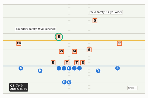
“Pass, incomplete, because the boundary safety rotated down and took away the out; QB stayed with it too long” is a good line. “Bad play” isn’t. If you can’t write the line, you haven’t seen the play yet: watch it again.

Why four passes, and not more

Why four, and not one per position? Because a fan’s eye can hold about one group at a time, and these four groups answer different questions in an order where each pass gives context to the next (watch the receivers first and you’ll call a receiver “open” who the quarterback never had time to look at). More passes add little: by pass 4 you’ve seen every player, and what’s left is re-watching the moment that matters, which you should do as often as you need. A snap takes about two minutes this way once you’re practised, more at first.

A full game, in the time you have

About 60 to 65 offensive snaps a side, at two minutes each, is more than four hours for both teams. Few people have that on a Monday. So run the protocol in layers:

  • Every snap: step 0 (freeze and check the pre-snap columns) and pass 3 (the coverage), because those are the two things the broadcast hid from you and your log’s second layer needs.
  • Every third down, red-zone snap, sack, turnover and explosive play: the full protocol. These are the snaps that decided the game, and there are usually 20 to 30 of them. (For an “explosive” use the analysts’ version from Expected Points and Success Rate, a run of 10 yards or more or a pass of 20 or more; staffs vary, and many count runs of 12 or more and passes of 16 or more.)
  • Everything else: at real speed once, then the chart row.

That’s two or three hours for one team’s offense against the other’s defense, which is a realistic weekly habit. (Coaches chart the kicking game too, every punt and kickoff; this chapter sticks to the snaps from scrimmage.)

Film room: one snap, four passes

NoteFilm room: Seahawks 2025 — Super Bowl LX, the strip-sack

The game: Seattle beat New England 29–13 in Super Bowl LX on February 8, 2026, at Levi’s Stadium in Santa Clara.3 Late in the third quarter Seattle led only 12–0, all on field goals, and New England had the ball.

The snap: third-and-6 at the New England 44, :16 left in the third quarter. The charting records the Patriots in 11 personnel in the shotgun with one back and motion before the snap; Seattle in its dime package (six defensive backs) with 6 in the box; 4 rushers; and coverage labelled 2-Man: man coverage underneath with two safeties deep (2-Man). Derick Hall sacked Drake Maye, forced a fumble, and Byron Murphy II recovered at the New England 37. Five snaps later Seattle scored its first touchdown, a 16-yard pass to AJ Barner, and led 19–0.4

Why this snap: it’s the question from the top of the chapter. A four-man rush got the sack; the film decides whether the rush won it or the coverage did.

The figure is a reconstruction in the same format as the course’s other replays: what was charted is exact, and the rest (who lined up where, the routes, which tackle Hall beat and how long it took) is a typical picture of that call, drawn to show what each pass of the protocol looks at. On the real film, you’d check every one of those details yourself.

Show the Python
def strip_sack():
    off = offense("gun_2x2")
    off = [p_.moved(w=1.5) if p_.key == "RB" else p_.moved(w=-18.5) if p_.key == "X" else p_ for p_ in off]
    dfn = [Player("HALL", "OLB", "def", 1.0, -7.4, label="58"), Player("DT", "DT", "def", 1.0, -1.0),
           Player("DE", "DE", "def", 1.0, 2.4), Player("OLB", "OLB", "def", 1.0, 6.0),
           Player("M", "ILB", "def", 5.0, 0.6, label="M"),
           Player("LCB", "CB", "def", 1.6, -17.6, label="CB"), Player("RCB", "CB", "def", 1.6, 14.2, label="CB"),
           Player("NB", "NB", "def", 3.4, -8.6), Player("DM", "DB", "def", 2.4, 8.2),
           Player("FS", "FS", "def", 12.5, -11.0), Player("SS", "SS", "def", 12.5, 9.0)]
    p = TrailPlay(off, dfn, los=54, to_go=6, ball_y="right")
    p.highlight("HALL")
    # the tight end motions across behind the line (well clear of the linemen) to a wing on the left; his man,
    # D, travels with him at linebacker depth and arrives at the same moment
    y_pts = [(-1.5, -5.0), (-1.5, -13.0), (0.5, -14.6)]                 # offsets from Y's spot (-1.5, 9.0)
    p.motion("Y", pts=y_pts, speed=5.0)
    y_len = float(np.hypot(1.5, 5.0) + 8.0 + np.hypot(2.0, 1.6))
    d_pts = [(0.4, -4.0), (0.4, -12.0), (0.6, -13.0)]                   # offsets from D's spot (2.4, 8.2)
    d_len = float(np.hypot(0.4, 4.0) + 8.0 + np.hypot(0.2, 1.0))
    p.motion("DM", pts=d_pts, speed=5.0 * d_len / y_len)
    for d_, rcv in (("LCB", "X"), ("NB", "H"), ("DM", "Y"), ("RCB", "Z")):
        p.trail_man(d_, rcv)                                             # trail technique: inside hip, underneath
    # offense: six block four. C and LG double the tackle, RG and RT take the right side one-on-one, the back
    # checks the A gap for a blitz and stays to help inside; the LT has Hall alone and rides him wide
    p.block("C", pts=[(-0.7, -0.3)]); p.block("LG", pts=[(-0.7, -0.1)])
    p.block("RG", pts=[(-0.9, 0.4)]); p.block("RT", pts=[(-1.2, 1.4)], speed=1.6)
    p.block("RB", pts=[(1.6, -1.9), (2.4, -2.5)], speed=2.4)
    p.block("LT", pts=[(-1.8, -1.2), (-3.7, -2.0), (-5.2, -2.0)], speed=1.7)
    # routes: a high-low on the left (H out at the sticks, Y in the flat under him), X clears deep, Z digs
    p.route("X", r.go(19)); p.route("H", r.out(7, 4)); p.route("Y", r.flat(2.0, 6.0), side=-1)
    p.route("Z", r.dig(12, 7))
    p.dropback(2.0)
    p.path("QB", [(1.0, -0.2)], speed=2.0, delay=1.4)                   # hitches up into the pocket
    p.read("Z")
    # defense: four rush, three of them held; Hall arcs past the launch point, then comes back under the tackle
    p.rush("DT", pts=[(-1.4, 0.1)], speed=0.9); p.rush("DE", pts=[(-1.4, 0.1)], speed=1.0)
    p.rush("OLB", pts=[(-2.0, -0.4)], speed=1.2)
    p.rush("HALL", pts=[(-3.2, -0.8), (-6.6, -0.4), (-8.6, 2.4), (-7.4, 6.2)], speed=4.3)
    p.drop("M", (4.5, -0.4), speed=2.0)                                  # the low hole, eyes on the quarterback
    p.drop("FS", (19.0, -14.0), speed=3.5); p.drop("SS", (19.0, 10.0), speed=3.5)
    return p


SSP = strip_sack()
T_SACK = 3.3
LAT_SS, WIN_SS = (-24, 21), (-10.5, 21.5)
animate_or_strip(SSP, [0.0, 1.5, 2.7, T_SACK],
                 ["Snap · Y motioned left; D went with him", "+1.5 s · two deep, four in man, M free",
                  "+2.7 s · QB climbs; the LT rides 58 wide", f"+{T_SACK} s · 58 comes back under: strip-sack"],
                 lateral=LAT_SS, window=WIN_SS)
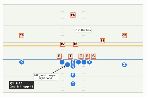
Figure 75.2: The strip-sack, third-and-6 (a reconstruction, simulated in Big Data Bowl format). Charted facts: 11 personnel in the shotgun with one back and motion; Seattle’s dime (six defensive backs), six in the box; four rushers; 2-Man (man coverage underneath, two safeties deep); a sack by Derick Hall (58, ringed), who forced a fumble. Illustrative: the alignments, the motion (here the tight end, Y, across to the left wing, with his defender, D, following him), the routes, the protection, and the time Hall took. What to notice: in the second panel every receiver has a defender a yard behind him and a yard inside, two safeties sit deep, and the middle linebacker (M) is free because the back stayed in; in the third the left tackle is still riding Hall wide as the quarterback climbs; in the fourth Hall has come back under the tackle to the quarterback.
Show the Python
T4 = 2.7
MAN_D = ["LCB", "NB", "DM", "RCB"]
PASSES = [
    ("Pass 1 · the line: 4 rushers, 6 blockers", ["LT", "LG", "C", "RG", "RT", "RB", "HALL", "DT", "DE", "OLB"], False,
     [("C + LG double the T;\nthe back helps inside", (-8.2, 12.5))], ()),
    ("Pass 2 · the QB: eyes right, hitch, no throw", ["QB"], True, [("2.7 s: still holding it", (-9.0, 11.5))], ()),
    ("Pass 3 · coverage: two deep, five under", MAN_D + ["M", "FS", "SS"], False,
     [("deep half", (15.6, -11.0)), ("deep half", (15.6, 10.0))], ()),
    ("Pass 4 · receivers: anyone open?", ["X", "H", "Y", "Z"], False, [("a defender on every route", (-9.0, 11.5))],
     MAN_D),
]
fig, axes = plt.subplots(2, 2, figsize=(6.5, 2 * (3.25 * (WIN_SS[1] - WIN_SS[0]) / (LAT_SS[1] - LAT_SS[0]) + 0.36)))
for ax, (title, keys, eyes, tags_, half_) in zip(axes.flat, PASSES):
    fld = snapshot(SSP, T4, ax, LAT_SS, WIN_SS)
    wash(fld, SSP, T4, keys, reads=eyes, half=half_)
    for txt, at in tags_:
        tag(fld, SSP, txt, at, fs=6.0)
    ax.set_title(title, fontsize=8.0, color=style.INK, loc="left")
fig.tight_layout(h_pad=0.5, w_pad=0.4)
plt.show()
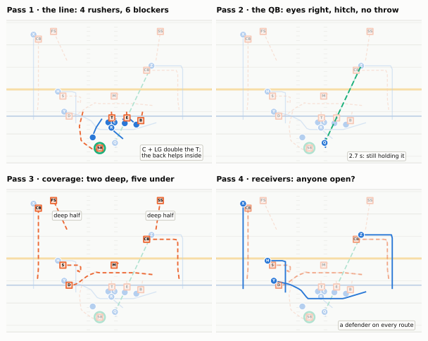
Figure 75.3: The same snap at 2.7 seconds, watched four times. Each panel fades everyone except the group that pass watches, with the paths they have run so far. Pass 1, the line: four rushers against five linemen and the back; the center and left guard double the tackle, the right side is one-on-one and holding, the back is helping inside, and Hall (58, ringed) has run wide and deep around the left tackle, who is still on him. Pass 2, the quarterback: a short drop, eyes to the right (the green dashed line), then a hitch up into the pocket. Pass 3, the coverage: both safeties in deep halves, the four man defenders a yard behind and inside their receivers (trail technique), and the middle linebacker (M) sitting in the short middle because the back stayed in to block. Pass 4, the skill players: four routes, each with a defender attached (drawn at half strength) and a safety above. A reconstruction, as in the previous figure.

Now run the protocol on it, the way you would on the real film.

Step 0, the freeze. Third-and-6 near midfield, down 12, sixteen seconds left in the third quarter: a pass, near certain. The offense is in 11 personnel in the shotgun; the defense in dime with six in the box and two safeties at about 12 yards. The motion is the useful clue: when the tight end crossed the formation, his defender went with him. That’s the man/zone indicator from Motion and Shifts voting man. A vote, not a verdict: Macdonald’s defenses disguise heavily and play plenty of match coverage (Fangio’s Two-High Revolution and Macdonald’s Answer), in which a defender can travel with a receiver too; and the other answer to watch for is a bump, the defenders sliding over a man each, which says zone or match. The two deep safeties say two-high. Put them together and the pre-snap read is 2-Man or a disguised rotation; on third-and-6 2-Man is a common answer, because it puts a defender on every receiver short of the sticks and two safeties over the top of them.

Pass 1, the line. Four rushers against six blockers (five linemen and the back). Ask where the two spares went: here the center and left guard double the tackle, and the back checks the gap in front of him for a blitzing linebacker, finds none, and stays to help inside. The right side holds one-on-one. That leaves the left tackle alone on Hall, which is normal: a tackle is expected to handle an edge rusher by himself for a few seconds. He does, riding Hall wide and deep past the quarterback’s launch point; the problem is that Maye climbs, and Hall comes back under. Count from the snap: in the reconstruction Hall arrives at about 3.3 seconds, in the shared zone between 2.5 and 3.5, where the line held long enough for the drop and the rest of the answer is in passes 2 to 4. The charting doesn’t record that time; on the real film it’s the first thing you’d measure.

Pass 2, the quarterback. Maye takes his drop, looks right, hitches up into the pocket and still doesn’t throw. That’s a quarterback with time and no answer, or one who missed an answer. Which, pass 4 will say.

Pass 3, the coverage. Both safeties pedal back and widen into deep halves. Underneath, every receiver has a defender a yard behind him and a yard inside, in trail technique, so anything short and inside is contested and anything deep has a safety coming. The middle linebacker has the back, and when the back stays in to block, he has a choice his coach gave him: add himself to the rush, or sit in the short middle as an extra defender. Here he sits, taking away the throw a quarterback looks for against man (the crossing route underneath) and, just as important, watching Maye. 2-Man’s great weakness is the quarterback scramble: every man defender has his back to the quarterback, so against a mobile one the linebacker in the low hole and the rushers’ lanes (who keeps him from escaping outside) are part of the coverage. Seven defenders in coverage against four receivers is the whole idea of rushing four: the rush doesn’t have to win quickly, because the coverage is designed to hold out.

Pass 4, the skill players. Against 2-Man, receivers need to win on their own: the route that beats it is the one that gets away from a trailing defender toward the sideline or back toward the quarterback, before the safety arrives. The drawn concept tries exactly that on the left, an out at the sticks over a flat underneath, with a dig on the right as the backside throw. At the moment Maye hitched, nobody had won. That’s the question to answer on the real film, frame by frame: was there a window at 2.5 seconds he passed up?

The “because” line. In this version: Sack because of the coverage: 2-Man took away everything inside and short of the sticks, the protection held for a normal drop, and the four-man rush won late, at 3.3 seconds, when the quarterback climbed into the edge rusher’s second move. If on the real film Hall had arrived in two seconds, it would read because the left tackle lost, and if a receiver had been open at 2.5 seconds, because the quarterback held it. Same play in the box score, three different lessons. That’s what the film is for.

CautionCommon misconception

“A sack is a pass-protection failure.” Often it isn’t. A sack is credited to the rusher who gets there, and the offensive line usually takes the blame, but a sack is the end of a chain: protection, quarterback, coverage, routes. A defense that rushes four and covers with seven is betting that its coverage will hold long enough for four rushers to win eventually, and when that bet pays off it’s a coverage sack. In Super Bowl LX Seattle rushed four on 45 of New England’s 53 dropbacks and got 5 of its 6 sacks that way. You can’t tell from the box score which of those were the line’s fault and which were the coverage’s. The film can. (And against a mobile quarterback the bet has a second half: the four rushers must keep their lanes, so the quarterback can’t escape the pocket while the coverage holds.)

Charting a game

The film tells you what happened on one snap. To learn what a team does, you need every snap in the same form, and that’s charting. Game charting means recording every snap of a game as one row of the same fixed fields (situation, personnel, formation, motion, the defense’s look, what happened after the snap, the result), coded the same way every time, so a game becomes data you can count. Everyone calls it charting for short.

You’ve been using other people’s charting since Part 13. When the participation file says a snap was Cover 6 against 11 personnel, somebody watched that snap and wrote those codes. NFL staffs do it too: their quality control coaches tag every snap of every opponent, and the tags become the tendency report (The Game Plan). Charting your own game puts you in that chair.

Why chart, when FTN and nflverse already do? Three reasons.

  1. Timing. The public charting doesn’t all arrive at once. The play-by-play for a game is usually available within hours; FTN’s charting (alignment, motion, play-action, rushers) arrives game by game during the season; but personnel and coverage labels, in the participation file, arrive only after the season ends, around February.5 If you want to know what coverage Seattle played against 12 personnel in this season, the public data can’t tell you until the season is over. Your chart can tell you tonight.
  2. What nobody publishes. The public files don’t record the pre-snap shell (only the coverage after the snap), the corners’ leverage, the formation’s strength, which way the run went relative to that strength, the run scheme, the pass concept, the routes of receivers who weren’t targeted, or who lost the block on a sack. Those are exactly the fields that make a tendency useful, and exactly what step 0 and the four passes record.
  3. The answer key. Your live log’s second layer (the coverage family, the rush, the direction of the run) needs something to be scored against. On a 2026 game, until the participation file arrives, your chart is the only answer key there is.

The charting sheet

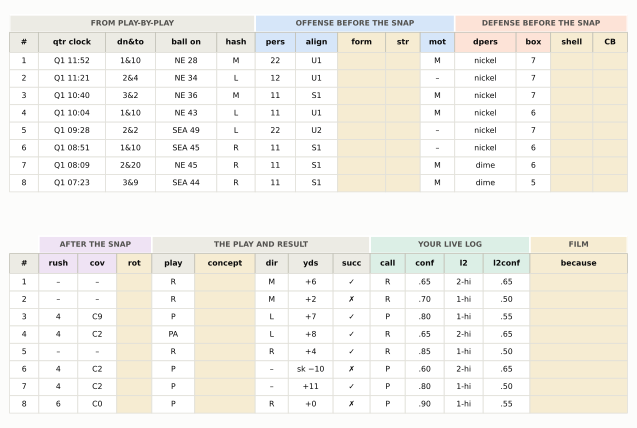
Here is the template. One row per snap, in seven blocks of columns:

Show the Python
SHEET = NE[NE.fixed_drive == NE.fixed_drive.min()].copy()
SHEET["l2conf"] = SHEET.down.map(lambda d_: conf_of(sea_two_rate(int(d_)), cap=0.9))
SHEET["l2"] = SHEET.down.map(lambda d_: "2-hi" if sea_two_rate(int(d_)) >= 0.5 else "1-hi")
SHEET["call"] = SB.set_index("play_id").loc[SHEET.play_id, "call"].values
SHEET["conf"] = SB.set_index("play_id").loc[SHEET.play_id, "conf"].values
SHEET = SHEET.reset_index(drop=True)


def dd(row, i=None):
    return f"{int(row['down'])}&{int(row['ydstogo'])}"


T1 = [("#", 3.0, "auto", lambda r_, i: str(i + 1)), ("qtr clock", 7.0, "auto", lambda r_, i: f"Q{int(r_['qtr'])} {r_['time']}"),
      ("dn&to", 5.2, "auto", dd), ("ball on", 6.4, "auto", lambda r_, i: r_["yrdln"]),
      ("hash", 4.0, "auto", lambda r_, i: r_["hash"]),
      ("pers", 4.2, "off", lambda r_, i: r_["pers"]), ("align", 4.4, "off", lambda r_, i: r_["align"]),
      ("form", 5.0, "film", None), ("str", 3.6, "film", None), ("mot", 3.6, "off", lambda r_, i: r_["mot"]),
      ("dpers", 6.4, "def", lambda r_, i: r_["dpers"]), ("box", 3.6, "def", lambda r_, i: r_["box"]),
      ("shell", 4.4, "film", None), ("CB", 3.6, "film", None)]
T2 = [("#", 3.0, "auto", lambda r_, i: str(i + 1)),
      ("rush", 4.0, "post", lambda r_, i: "–" if pd.isna(r_["rush"]) or r_["qb_dropback"] != 1 else str(int(r_["rush"]))),
      ("cov", 4.0, "post", lambda r_, i: r_["cv"] if isinstance(r_["cv"], str) else "–"), ("rot", 3.6, "film", None),
      ("play", 4.4, "auto", lambda r_, i: r_["kind"]), ("concept", 6.2, "film", None),
      ("dir", 3.4, "auto", lambda r_, i: {"left": "L", "middle": "M", "right": "R"}.get(
          r_["pass_location"] if r_["qb_dropback"] == 1 else r_["run_location"], "–")),
      ("yds", 4.6, "auto", lambda r_, i: r_["res"]), ("succ", 3.8, "auto", lambda r_, i: "✓" if r_["success"] == 1 else "✗"),
      ("call", 3.6, "log", lambda r_, i: r_["call"]), ("conf", 4.0, "log", lambda r_, i: f"{r_['conf']:.2f}".lstrip("0")),
      ("l2", 4.0, "log", lambda r_, i: r_["l2"]), ("l2conf", 4.8, "log", lambda r_, i: f"{r_['l2conf']:.2f}".lstrip("0")),
      ("because", 10.0, "film", None)]
FILL = {"auto": AUTO_TINT, "off": style.OFFENSE_TINT, "def": style.DEFENSE_TINT, "post": "#efe3f4", "log": LOG_TINT,
        "film": FILM_TINT}
GROUPS1 = [("FROM PLAY-BY-PLAY", 0, 5, "auto"), ("OFFENSE BEFORE THE SNAP", 5, 10, "off"),
           ("DEFENSE BEFORE THE SNAP", 10, 14, "def")]
GROUPS2 = [("AFTER THE SNAP", 1, 4, "post"), ("THE PLAY AND RESULT", 4, 9, "auto"), ("YOUR LIVE LOG", 9, 13, "log"),
           ("FILM", 13, 14, "film")]
nr = len(SHEET)
RH, HH, GH = 1.0, 1.15, 1.0
tier_h = GH + HH + RH * nr
fig, axes = plt.subplots(2, 1, figsize=(6.5, 2 * 0.2 * (tier_h + 0.6)))
for ax, cols, groups in ((axes[0], T1, GROUPS1), (axes[1], T2, GROUPS2)):
    blank(ax)
    Wt = sum(w for _, w, _, _ in cols)
    ax.set_xlim(0, Wt)
    ax.set_ylim(-0.3, tier_h + 0.3)
    xs = np.cumsum([0] + [w for _, w, _, _ in cols])
    for name, a, b, kind in groups:
        ax.add_patch(Rectangle((xs[a], tier_h - GH), xs[b] - xs[a], GH, fc=FILL[kind], ec="white", lw=1.2))
        ax.text((xs[a] + xs[b]) / 2, tier_h - GH / 2, name, ha="center", va="center", fontsize=5.6,
                fontweight="bold", color=style.INK_2)
    yh = tier_h - GH - HH
    for j, (name, w, kind, fn) in enumerate(cols):
        ax.add_patch(Rectangle((xs[j], yh), w, HH, fc=FILL[kind], ec=style.BASELINE, lw=0.6))
        ax.text(xs[j] + w / 2, yh + HH / 2, name, ha="center", va="center", fontsize=5.8, fontweight="bold",
                color=style.INK)
        for i_, (_, row) in enumerate(SHEET.iterrows()):
            yy = yh - (i_ + 1) * RH
            ax.add_patch(Rectangle((xs[j], yy), w, RH, fc=FILM_TINT if fn is None else "white", ec=style.GRID,
                                   lw=0.6))
            if fn is not None:
                ax.text(xs[j] + w / 2, yy + RH / 2, fn(row, i_), ha="center", va="center", fontsize=5.8,
                        color=style.INK)
fig.subplots_adjust(left=0.005, right=0.995, top=0.995, bottom=0.005, hspace=0.18)
plt.show()
Figure 75.4: The charting sheet, with New England’s first eight snaps of Super Bowl LX filled in from public data. The sheet is one long row per snap, printed here in two tiers that share the snap number (#). Grey blocks fill themselves from the play-by-play. The blue block (the offense before the snap), the peach block (the defense before the snap) and the lavender block (after the snap) are what you chart from film, filled here from FTN’s charting and the participation file where those record the field. Cream-shaded cells are fields no public source records (formation, strength, the pre-snap shell, the corners, the rotation, the play concept, the ‘because’ line), which only your own film can fill. The green block is your live log, filled here with calls made by rule from the pre-snap columns (as in Watching Live), standing in for yours: a run-or-pass call and its confidence, then a second-layer call (l2) on whether Seattle would play two-high or one-high and its confidence (l2conf), made from Seattle’s 2025 rate for the down. Every column is decoded in the codebook below.

And here is the codebook that goes with it. The codes matter less than the rule behind them: decide them before you start, write them on the sheet, and use them the same way on every snap. A chart in which “Cover 3” meant one thing in the first quarter and another in the fourth can’t be counted.

Table 75.1: The codebook for the charting sheet. ? is always allowed and is better than a guess. The last column says whether a careful viewer can usually fill the field from the broadcast alone: ✓ yes, “some” on most snaps, “rarely” only when a replay happens to show it.
Column Codes The rule TV?
qtr clock Q1 15:00 Quarter and game clock at the snap ✓
dn&to 3&6 Down and yards to go ✓
ball on NE 44 The ball’s spot (the side of the field, then the yard line) ✓
hash L, M, R Where the ball was spotted: left hash, middle, right hash ✓
pers 11, 12, 21, 13, 10, 22 … Backs, then tight ends; count as they run on ✓
align U, S or P plus the number of backs: U1, S0, P1 Where the quarterback stands, how many in the backfield ✓
form 2x2, 3x1, bunch, empty 3x2, I, offset I … Pick one name per look and reuse it some
str L, R The strong side, by one rule you write at the top of the sheet (tight end, receivers, or field) some
mot –, M (motion), S (shift), J (still moving at the snap) What moved, and when ✓
dpers base, nickel, dime Count the defensive backs some
box a number Defenders in the box (from just outside the end men on the line, about 5 to 7 yards deep), counted at the snap, after any motion some
shell 0, 1, 2 Deep safeties at the snap (before any rotation) rarely
CB P or O, plus i or o Press or off; inside or outside leverage rarely
rush a number Rushers after the snap some
cov C0, C1, C2, 2M, C3, C4, C6, C9, ? The coverage played after the snap rarely
rot –, B, F; add * if late (B*) Rotation: none, to the boundary, to the field; the star marks one that started at or after the snap rarely
play R, P, PA, SCR, RPO Run, dropback, play-action, screen, run-pass option; a scramble is a dropback (P), a designed quarterback run is a run (R) ✓
concept IZ, OZ, PWR, CTR, DUO, TRAP, TOSS, ZR (zone read), QB (designed QB run); smash, flood, mesh, stick … The run scheme or pass concept, in the course’s names some
dir L, M, R Where the run hit or the pass went ✓
yds +7, −3, sk −7, INT, FUM, TD The result: yards, a sack, a turnover or a score ✓
succ ✓ or ✗ A successful play: positive EPA, nflverse’s success flag (Expected Points and Success Rate) ✓
call, conf P or R; 0.50 to 0.90 Your live log: the run-or-pass call and its stated confidence ✓
l2, l2conf 2-hi, 1-hi, zone, man, 5+, left …; 0.50 to 0.90 Your live log’s second-layer call and its confidence (how sure you were of that call, as for conf) ✓
because free text One line from the protocol: whose play it was

Three rules keep a chart honest:

  • ? is a code. If the broadcast cut away, or you can’t tell Cover 1 from Cover 3 on a late rotation, write ?. A guessed label looks exactly like a real one in the totals and quietly poisons them.
  • Code what you see, not what you expect. Charting a team you’ve studied, you’ll be tempted to write its favourite coverage before you’ve watched the safeties. That’s how a tendency becomes a self-fulfilling one in your chart.
  • Never edit the live log. The chart is what happened; the log is what you knew before it happened. Keep them in separate columns and score one against the other.

The skeleton: let the play-by-play do the typing

A third of the sheet is already known before you press play: the snap order, the clock, down and distance, the ball’s spot, the result. nflverse publishes all of it within hours of each game, so the sensible way to start a chart is to build the skeleton in code and spend your film time only on what the film adds. This function does it for any game in any season nflverse covers:

import numpy as np
import pandas as pd
from gridiron.data import pbp

FILM_COLUMNS = ["pers", "align", "form", "str", "mot", "dpers", "box", "shell", "CB",
                "rush", "cov", "rot", "concept", "because", "notes"]


def chart_skeleton(game_id, team):
    """One row per snap of `team`'s offense, with the play-by-play columns filled and the film columns empty."""
    season = int(game_id[:4])
    d = pbp([season])
    d = d[(d.game_id == game_id) & (d.posteam == team) & d.play_type.isin(["pass", "run"])
          & d.down.notna()]               # a two-point try has no down; it isn't a charted snap
    sheet = pd.DataFrame({
        "play_id": d.play_id.astype(int), "qtr": d.qtr.astype(int), "clock": d.time,
        "down": d.down.astype(int), "togo": d.ydstogo.astype(int), "ball_on": d.yrdln,
        "play": np.where(d.qb_dropback == 1, "P", "R"),        # scrambles and sacks are dropbacks
        "dir": d.pass_location.fillna(d.run_location).str[0].str.upper(),
        "yds": d.yards_gained.astype(int), "success": d.success.astype(int), "epa": d.epa.round(2)})
    for c in FILM_COLUMNS:
        sheet[c] = ""                     # yours to fill from the film
    return sheet.reset_index(drop=True)


sheet = chart_skeleton("2025_22_SEA_NE", "NE")          # Super Bowl LX, New England's offense
print(f"{len(sheet)} snaps; first five of the play-by-play half:")
print(sheet.iloc[:5, :11].to_string(index=False))
66 snaps; first five of the play-by-play half:
 play_id  qtr clock  down  togo ball_on play dir  yds  success   epa
     279    1 11:52     1    10   NE 28    R   M    6        1  0.28
     301    1 11:21     2     4   NE 34    R   M    2        0 -0.37
     323    1 10:40     3     2   NE 36    P   L    7        1  1.15
     353    1 10:04     1    10   NE 43    P   L    8        1  0.58
     378    1 09:28     2     2  SEA 49    R   R    4        1  0.25

The skeleton is the blank template: save it with sheet.to_csv("sb60_ne.csv", index=False), open it in a spreadsheet next to the film, and the empty columns, in the codebook’s order, are the ones to fill. (Penalties that wipe out a snap, kneels and spikes aren’t in it; add a row by hand if a wiped-out snap told you something.) For a current-season game, the same call gives you the skeleton within hours of the game, weeks or months before the public coverage labels exist.

Is your chart any good?

Professional charters disagree with each other, and you’ll disagree with yourself. The cheap test is to chart one quarter twice, a week apart, without looking at the first attempt, and compare. For each film column, count how often the two attempts agree. Personnel and the box should agree almost every time; if they don’t, your definition is fuzzy (where exactly does “the box” end?). Coverage will agree less often, and that’s normal: it’s the hardest column, and the place to use ? more freely. If you want a single number that allows for agreement by chance, Cohen’s kappa is the standard one.6 You don’t need it to learn something: the columns where you disagree with yourself are the ones to stop trusting in your totals, and the ones to practise.

Film room: a whole game, charted

NoteFilm room: Seahawks 2025 — Super Bowl LX, charted end to end

The game: Seahawks 29, Patriots 13, Super Bowl LX. In 2025 Seattle’s head coach was Mike Macdonald, its offensive coordinator Klint Kubiak and its defensive coordinator Aden Durde; New England’s offensive coordinator was Josh McDaniels.7 The Game Plan rebuilt, from public charting, the tendency report New England’s staff might have read about Seattle’s defense before this game. This is the game itself.

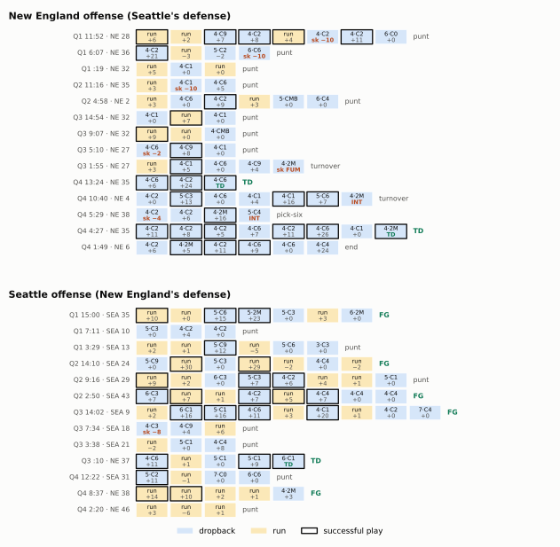
The chart: every one of the game’s 137 runs and dropbacks, both offenses, in the sheet’s codes, filled from the public charting (play-by-play, FTN and the participation file, which covers the playoffs).8 The film-only columns are left empty: they’re yours.

What to notice: how much of the game’s story is visible in the rows, and how much isn’t.

Show the Python
RES_TXT = {"Punt": "punt", "Field goal": "FG", "Touchdown": "TD", "Turnover": "turnover", "Opp touchdown": "pick-six",
           "End of half": "end", "Missed field goal": "missed FG", "Turnover on downs": "downs"}


def board(ax, T, title):
    drives = list(dict.fromkeys(T.fixed_drive))
    nmax = 10
    CW, RH_ = 1.0, 1.0
    LW_ = 3.7
    ax.set_xlim(-LW_, nmax * CW + 2.2)
    ax.set_ylim(len(drives) + 0.15, -1.25)
    blank(ax)
    ax.text(-LW_, -0.75, title, fontsize=8.2, fontweight="bold", color=style.INK, va="center")
    for i_, dv in enumerate(drives):
        Dd = T[T.fixed_drive == dv]
        r0 = Dd.iloc[0]
        ax.text(-0.15, i_ + 0.5, f"Q{int(r0.qtr)} {r0.time.lstrip('0')} · {r0.yrdln}", ha="right", va="center",
                fontsize=5.6, color=style.INK_2)
        for j, (_, row) in enumerate(Dd.iterrows()):
            x0 = j * CW
            is_p = row.qb_dropback == 1
            fc = style.OFFENSE_TINT if is_p else "#fbe8b8"
            ok = row.success == 1
            ax.add_patch(Rectangle((x0 + 0.04, i_ + 0.06), CW - 0.08, RH_ - 0.12, fc=fc,
                                   ec=style.INK if ok else "white", lw=1.0 if ok else 0.4))
            if is_p:
                ru = "–" if pd.isna(row.rush) else str(int(row.rush))
                cv = row.cv if isinstance(row.cv, str) else "–"
                top = f"{ru}·{cv}"
            else:
                top = "run"
            ax.text(x0 + CW / 2, i_ + 0.34, top, ha="center", va="center", fontsize=4.9, color=style.INK)
            bad = row.res.startswith("sk") or row.res in ("INT", "FUM")
            ax.text(x0 + CW / 2, i_ + 0.72, row.res, ha="center", va="center", fontsize=4.9,
                    color=style.DEFENSE_DARK if bad else (LOOK if row.res == "TD" else style.INK_2),
                    fontweight="bold" if (bad or row.res == "TD") else "normal")
        res = RES_TXT.get(r0.fixed_drive_result, str(r0.fixed_drive_result).lower())
        ax.text(len(Dd) * CW + 0.15, i_ + 0.5, res, ha="left", va="center", fontsize=5.8,
                color=LOOK if res in ("TD", "FG") else style.INK_2, fontweight="bold" if res in ("TD", "FG") else "normal")


nd_ne, nd_sea = NE.fixed_drive.nunique(), SEA.fixed_drive.nunique()
fig, (a1, a2) = plt.subplots(2, 1, figsize=(6.5, 0.205 * (nd_ne + nd_sea + 4.2)),
                             gridspec_kw=dict(height_ratios=[nd_ne + 1.4, nd_sea + 1.4]))
board(a1, NE, "New England offense (Seattle's defense)")
board(a2, SEA, "Seattle offense (New England's defense)")
handles = [Patch(fc=style.OFFENSE_TINT, ec="none", label="dropback"), Patch(fc="#fbe8b8", ec="none", label="run"),
           Patch(fc="white", ec=style.INK, lw=1.0, label="successful play")]
a2.legend(handles=handles, loc="upper center", bbox_to_anchor=(0.5, 0.0), ncol=3, fontsize=6.6, frameon=False)
fig.subplots_adjust(left=0.01, right=0.99, top=0.99, bottom=0.05, hspace=0.12)
plt.show()
Figure 75.5: Super Bowl LX on one page: every run and dropback, one cell per snap, one row per drive, New England’s offense on top and Seattle’s below. Blue cells are dropbacks (including sacks and scrambles), amber cells runs; a dark outline marks a successful play (one with positive EPA: it left the offense better placed to score than before the snap). For dropbacks the top line gives the number of rushers and the charted coverage (2M = 2-Man, C6 = Cover 6, and so on; ‘–’ where none was charted); for runs it says ‘run’. The bottom line is the result: yards, a sack, an interception (INT), a lost fumble (FUM) or a touchdown (TD). The right-hand label is how the drive ended. What to notice: the Patriots’ first nine drives, none longer than eight snaps, eight ending in punts and the ninth in the strip-sack, against a defense rushing four on almost every dropback and playing two-deep behind it; and Seattle’s offense, steady rather than explosive, turning four of its first seven drives into field goals. Source: nflverse play-by-play, FTN charting and participation, game 2025_22_SEA_NE.

Now read the chart the way a coach reads a tendency report: count, then ask why.

What the charted Super Bowl says, set against the teams’ regular-season habits (Seattle’s defense, unless the row says otherwise) and the league’s. Two-high counts Cover 2, 2-Man, Cover 4 and Cover 6; the labelled dropbacks exclude the snaps FTN coded as COMBO. Pressure is the participation file’s was_pressure flag on dropbacks, the same definition in every column. Source: nflverse play-by-play, FTN charting and participation; course calculation.
From the chart Super Bowl LX 2025 regular season League, 2025
New England dropbacks with four rushers 45 of 53 (85%) 76% 70%
Two-high coverage after the snap (of labelled dropbacks) 73% (51 labelled) 52% 43%
Man coverage (of dropbacks charted man or zone) 28% — —
Pressure on New England dropbacks 28% 34% 30%
Sacks; with four rushers 6; 5 — —
New England snaps that were dropbacks 80% of 66 New England: 60% —
Seattle snaps that were runs 44% of 71 Seattle: 48% —
Kenneth Walker III 27 carries, 135 yards — —

Four things jump out of those rows.

Seattle did in the biggest game what it did all season, only more so. Rushing four and playing two deep behind it was Seattle’s identity (Fangio’s Two-High Revolution and Macdonald’s Answer), and the Super Bowl chart is that identity turned up: four rushers on 85% of dropbacks and two-high on 73% of the labelled ones. A tendency report told New England this was coming. Knowing it and beating it are different things.

The four-man rush didn’t pressure more often; it finished. Seattle pressured Maye on 28% of dropbacks, no more than its regular-season rate (34%) or the league’s (30%). What changed was what pressure turned into: 6 sacks, 5 of them with four rushers. That’s the “coverage holds, rush wins late” bet from the strip-sack paying off across a whole game: when the coverage leaves nowhere to throw, ordinary pressure becomes sacks. It’s also the kind of claim only film can settle, snap by snap.

The scoreboard shaped the play-calling. New England dropped back on 80% of its snaps, against 60% in its regular season, because it trailed from the first quarter on and spent the fourth quarter chasing three scores. Read that number as a tendency and you’d call New England’s offense pass-happy; it was a game state. Seattle, ahead all night, ran on 44% of its snaps (its season rate: 48%), with Kenneth Walker III carrying 27 times. The neutral-situation filter of Tendencies exists for exactly this reason. One game’s chart describes that game, not the team.

And the chart is silent where the film isn’t. The public rows can’t tell you which of New England’s two-high looks were shown before the snap and which were played after it, which receivers Seattle’s man defenders were matched on, or who lost the block on each sack. Those are the cream-shaded columns of the sheet, and they’re where the answers to “how did Seattle do it?” live. A full chart of this game, with the film columns filled, is a weekend’s project and the best one this chapter can offer you.

From rows to tendencies

Counting a chart is a few lines of pandas. Start from the skeleton, fill the film columns (here two of them, the coverage and the rush, are filled from the participation file so the example runs; on your own chart you’d have typed them), and ask the chart a question in the form how often is it this, when it’s that?

from gridiron.data import nfl

# The skeleton from above, with two film columns filled from the public labels (stand-ins for your own film)
part = nfl().load_participation([2025]).to_pandas()
part = part[part.nflverse_game_id == "2025_22_SEA_NE"]
part = pd.DataFrame({"play_id": part.play_id.astype(int), "cov": part.defense_coverage_type,
                     "rush": part.number_of_pass_rushers.astype("Int64")})
chart = sheet.drop(columns=["cov", "rush"]).merge(part, on="play_id", how="left")

TWO_HIGH_CODES = {"COVER_2", "2_MAN", "COVER_4", "COVER_6"}
ONE_HIGH_CODES = {"COVER_0", "COVER_1", "COVER_3", "COVER_9"}
chart["shell_played"] = np.select([chart["cov"].isin(TWO_HIGH_CODES), chart["cov"].isin(ONE_HIGH_CODES)],
                                  ["2-hi", "1-hi"], default="?")


def tendency(chart, by, col):
    """For each value of `by`, the share of snaps with each code in `col`, and how many snaps that is."""
    t = pd.crosstab(chart[by], chart[col], normalize="index").round(2)
    t["snaps"] = chart[by].value_counts()
    return t


drops = chart[chart.play == "P"]
print("Seattle's coverage shell against New England's dropbacks, by down:")
print(tendency(drops, "down", "shell_played").to_string())
print("\nSeattle's rushers, by down:")
print(tendency(drops[drops.rush.fillna(0) > 0], "down", "rush").to_string())
Seattle's coverage shell against New England's dropbacks, by down:
shell_played  1-hi  2-hi     ?  snaps
down                                 
1             0.10  0.90  0.00     20
2             0.37  0.58  0.05     19
3             0.36  0.57  0.07     14

Seattle's rushers, by down:
rush     4     5     6  snaps
down                         
1     0.90  0.10  0.00     20
2     0.84  0.16  0.00     19
3     0.79  0.00  0.21     14

Two lines of output and you have the start of a tendency report: what Seattle played, and how many it sent, on each down. With your own film columns filled, the same function asks the questions no public file can. tendency(drops, "shell", "shell_played") is shown against played: how often a two-high shell at the snap stayed two-high. tendency(chart[chart.play == "R"], "str", "dir") is how often the runs went to the strength. tendency(chart, "pers", "form") is what each personnel group lines up in. Keep the snaps column in view: a share from five snaps is a hint, not a tendency, which is the same small-sample warning Tendencies gave about the public data.

CautionCommon misconception

“The chart is the truth about the game.” A chart is a record of one charter’s judgements, coded consistently. It’s far better than memory and far better than the box score, but its coverage column is an inference from film, its box count depends on where you draw the box, and its “because” line is an opinion. Treat a chart the way Tendencies taught you to treat FTN’s: strong evidence about habits across many snaps, weaker evidence about any single one.

Scoring yourself

Now the log. Since Downs, Distance, and Field Position you’ve been calling run or pass before the snap. Since How to Watch a Broadcast you’ve written a confidence next to each call, and since Watching Live that confidence has been a stated number between 50% and 90%. This section scores it.

To make that concrete, the rest of the chapter uses an example log: every Panthers offensive snap of the 2025 season, 1054 calls across 18 games (17 regular-season games and the wild-card loss to the Rams). The situations and the results are real. The calls are simulated: a reader who sees roughly what a model using the situation and the formation sees, through some noise, and who starts the season overconfident and settles down as it goes on.9 It’s a stand-in for your log, built so that its mistakes are the common ones. Its clue column uses just two codes, so it can be counted: align on snaps where the formation moved the call away from what the situation alone said (where the situation-and-formation model and xpass differ by more than ten points), and sit where the situation alone decided it. (In Watching Live the clue column was free text; settling on a few codes is what lets you score it.) On the website, the folded code at the top of the chapter builds this log; LOGDF.to_csv("prediction_log_2025.csv", index=False) writes it out if you want to run what follows.

Why hit rate isn’t enough

The first number is the one you’ve been computing since Part 1: the share of calls that came true. The example reader was right on 74% of calls. Against the bars from How to Watch a Broadcast, that’s good: on the same Panthers snaps, “always pass” would have been right 59% of the time, the down-and-distance rule from your first tally 60%, and nflverse’s situation-only xpass model 66%.

But hit rate throws away the confidence column, and the confidence column is where most of a reader’s skill shows. Two readers can both be right 70% of the time: one who said 70% on every call and meant it, and one who said 95% on half his calls and 55% on the rest and was wrong on a pile of the 95s. The second reader is making a mistake the hit rate can’t see. You need a score that rewards being right and being honest about how sure you were.

The Brier score

That score is the Brier score: the average, over all your calls, of the squared gap between your stated confidence and what happened, counting what happened as 1 if the call came true and 0 if it didn’t.

\[ \text{Brier} = \frac{1}{N}\sum_{i=1}^{N} \left(c_i - o_i\right)^2, \qquad c_i = \text{stated confidence},\quad o_i = \begin{cases}1 & \text{call came true}\\ 0 & \text{it didn't}\end{cases} \]

Lower is better. Three calls make the arithmetic plain:

Three calls, scored. The confident miss costs twenty times what the confident hit earned back.
Call Confidence Came true? Gap Squared
Pass 0.80 yes (1) 0.20 0.04
Run 0.60 no (0) 0.60 0.36
Pass 0.90 no (0) 0.90 0.81
Brier (0.04 + 0.36 + 0.81) / 3 = 0.40

Read the table as a set of incentives. A confident call that comes true costs almost nothing (0.04). A timid call that misses costs a moderate amount (0.36). A confident call that misses costs a lot (0.81). And a reader who says 50% on every snap, never committing to anything, scores exactly 0.25, whatever happens, because every gap is one half. So 0.25 is the “I have nothing” line: a log that scores worse than 0.25 has done harm by stating its confidences.

Glenn Brier, a statistician and meteorologist at the U.S. Weather Bureau, proposed the score in 1950 to grade forecasts like “70% chance of rain”, and it’s still the standard way to grade probability forecasts in weather, in medicine, and in the forecasting tournaments that taught Watching Live its habit of stating numbers.10 It doesn’t matter which way round you write your calls: scoring “pass, 0.70” against whether it was a pass gives the same number as scoring “my call, 0.70” against whether your call came true. Your log’s conf and hit columns are all it needs.

Why squared? A score you can’t game

Why square the gap, rather than just averaging it, or awarding points for confidence on the calls you got right? Because of what each rule rewards you for saying. Suppose that on a certain kind of snap, a call comes true 75% of the time, and you know it. What should you say?

Show the Python
cs = np.linspace(0.5, 1.0, 101)
fig, (a1, a2) = plt.subplots(1, 2, figsize=(6.5, 2.6))
for q, col in zip((0.6, 0.75, 0.9), (style.SERIES[0], style.SERIES[1], style.SERIES[2])):
    a1.plot(cs, q * (1 - cs) ** 2 + (1 - q) * cs ** 2, color=col, lw=1.8, label=f"calls that come true {int(q * 100)}% of the time")
    a1.scatter([q], [q * (1 - q)], color=col, s=26, zorder=4, edgecolor="white", linewidth=0.8)
    a2.plot(cs, q * cs, color=col, lw=1.8)
a1.set_xlim(0.5, 1.0)
a1.set_ylim(0, 0.42)
a1.set_title("Brier score: say what you believe", fontsize=8.2)
a1.set_ylabel("expected score per call (lower is better)", fontsize=6.8)
a2.set_xlim(0.5, 1.0)
a2.set_ylim(0.25, 0.95)
a2.set_title("'Points for confidence': always say 100%", fontsize=8.2)
a2.set_ylabel("expected points per call (higher is better)", fontsize=6.8)
for a in (a1, a2):
    a.set_xlabel("the confidence you state", fontsize=7.0)
    a.xaxis.set_major_formatter(plt.FuncFormatter(lambda v, _: f"{v:.0%}"))
    a.tick_params(labelsize=6.6)
fig.legend(*a1.get_legend_handles_labels(), loc="lower center", ncol=3, fontsize=6.6, frameon=False)
fig.tight_layout(w_pad=2.0, rect=(0, 0.08, 1, 1))
plt.show()
Figure 75.6: Why the Brier score squares the gap. Each curve is the score you should expect, call after call, if you always state the confidence on the horizontal axis on snaps where your call really comes true 60%, 75% or 90% of the time. Left, the Brier score (lower is better): every curve bottoms out exactly at the true rate (the dots), so the best thing you can do is say what you believe. Right, a naive rule that awards your stated confidence as points when you’re right and nothing when you’re wrong (higher is better): every line rises to the right edge, so it pays you to say 100% on every call, whatever you believe. A scoring rule with the Brier score’s property is called proper.

That property has a name: the Brier score is a proper scoring rule. Its expected value is lowest when you state exactly the probability you believe, so there’s no way to game it by shading your numbers up or down. The curves also explain the advice in Watching Live to rarely go above 90%: near the bottom each curve is flat, and away from it it climbs fast. On the 75% curve, saying 80% instead of 75% costs 0.0025 a call; saying 100% costs 0.0625, twenty-five times as much.

Skill: compared with what?

A Brier score means little on its own; 0.19 is good or bad depending on how predictable the snaps were. So compare it with forecasters who know less than you, on the same snaps. On the Panthers’ 2025 snaps:

The example log against honest baselines, on the same Panthers snaps. xpass is nflverse’s model (trained on the 2006–2019 seasons, so it has never seen these snaps either); the last row is the situation-and-formation model from Watching Live’s steps 1 to 3, learned on 2024. Course calculation from nflverse play-by-play and FTN charting.
Forecaster What it knows Brier score
Always 50% Nothing 0.250
The base rate The Panthers threw on 59% of snaps; says that every time 0.241
xpass The situation on the scorebug: down, distance, field position, score, clock 0.205
The example reader What the reader saw, as logged 0.186
Situation + formation model The situation, plus the quarterback’s alignment and the number of backs 0.175

The Brier skill score turns a comparison into one number: one minus the ratio of your score to the reference’s. Against the base rate, the example reader’s skill is 0.23, meaning the log removed about 23% of the error of a forecaster who only knew the team’s pass rate. Against xpass it’s 0.09: the reader beat “the scorebug” (xpass knows only what the scorebug shows: down, distance, field position, score and clock), because the formation was working for him. And the last row is the bar for a reader who uses only those two clues, the situation and the formation; the box, the shell and the tells of Watching Live can take a reader past it. The gap between the reader and that row is the room left with those two clues: some of it is calibration (stating the right number), some of it is the noise of reading a broadcast in twenty seconds.

There’s no published table of what a “good fan” scores, and it would mean little if there were, because the number depends on the snaps: a team that runs on every short-yardage down is easier to read than one that doesn’t. Your bars are the baselines on your own snaps.

That’s the comparison to make with your own log. Beat 0.25 and your confidences are doing more good than harm. Beat the base rate and you know more than the team’s tendency. Beat xpass and you’re reading something the scorebug doesn’t show.

Calibration

The Brier score says how good. The calibration plot says which way to adjust. Calibration is how closely your stated confidences match how often your calls come true: a well-calibrated reader’s 70% calls come true about 70% of the time, his 90% calls about 90%. To see it, group your calls by the confidence you stated, and for each group plot the stated confidence against the share that actually came true. Perfect calibration is the diagonal.

Show the Python
def bins(conf):
    return pd.cut(conf, [0.49, 0.575, 0.675, 0.775, 0.875, 1.0], labels=False)


def wilson(k, n, z=1.96):
    if n == 0:
        return np.nan, np.nan
    p = k / n
    den = 1 + z ** 2 / n
    mid = (p + z ** 2 / (2 * n)) / den
    half = z * np.sqrt(p * (1 - p) / n + z ** 2 / (4 * n ** 2)) / den
    return mid - half, mid + half


def calib_table(conf, hit):
    t = pd.DataFrame({"c": conf, "h": hit, "b": bins(np.asarray(conf))})
    g = t.groupby("b").agg(n=("h", "size"), k=("h", "sum"), c=("c", "mean"), h=("h", "mean")).reset_index()
    lohi = np.array([wilson(k, n) for k, n in zip(g.k, g.n)])
    g["lo"], g["hi"] = lohi[:, 0], lohi[:, 1]
    return g


fig = plt.figure(figsize=(6.5, 4.3))
axm = fig.add_axes([0.1, 0.33, 0.62, 0.62])
axc = fig.add_axes([0.1, 0.08, 0.62, 0.17], sharex=axm)
axm.plot([0.5, 1.0], [0.5, 1.0], color=style.INK_2, lw=1.0, ls=(0, (3, 2)), zorder=1)
axm.text(0.955, 0.985, "perfect", fontsize=6.6, color=style.INK_2, ha="right", va="center", rotation=36)
SERIES = [("games 1–8", FIRST, style.SERIES[1], -0.006), ("games 9–18", ~FIRST, style.SERIES[0], 0.006)]
for lab, m, col, dx in SERIES:
    g = calib_table(ME_CONF[m], HIT[m])
    axm.vlines(g.c + dx, g.lo, g.hi, color=col, lw=1.4, alpha=0.75, zorder=2)
    axm.plot(g.c + dx, g.h, color=col, lw=1.4, marker="o", ms=5.5, mec="white", mew=0.8, zorder=3)
    axc.bar(g.c + dx * 1.6, g.n, width=0.018, color=col, zorder=2)
axm.set_xlim(0.47, 1.0)
axm.set_ylim(0.4, 1.0)
axm.set_ylabel("how often the calls came true", fontsize=7.4)
axm.yaxis.set_major_formatter(plt.FuncFormatter(lambda v, _: f"{v:.0%}"))
axm.tick_params(labelbottom=False, labelsize=6.8)
axc.set_ylabel("calls", fontsize=7.0)
axc.set_xlabel("the confidence stated", fontsize=7.4)
axc.xaxis.set_major_formatter(plt.FuncFormatter(lambda v, _: f"{v:.0%}"))
axc.tick_params(labelsize=6.6)
axc.grid(axis="x", visible=False)
fig.text(0.75, 0.9, "Games 1–8", color=style.SERIES[1], fontsize=8, fontweight="bold")
fig.text(0.75, 0.855, f"Brier {ME['b1']:.3f}\nright {pct(ME['a1'])}, said {pct(ME['c1'])}", color=style.INK, fontsize=7,
         va="top", linespacing=1.3)
fig.text(0.75, 0.72, "Games 9–18", color=style.SERIES[0], fontsize=8, fontweight="bold")
fig.text(0.75, 0.675, f"Brier {ME['b2']:.3f}\nright {pct(ME['a2'])}, said {pct(ME['c2'])}", color=style.INK,
         fontsize=7, va="top", linespacing=1.3)
fig.text(0.75, 0.52, "Below the diagonal:\noverconfident.\nAbove it:\nunderconfident.", color=style.INK_2, fontsize=6.8,
         va="top", linespacing=1.3, style="italic")
plt.show()
Figure 75.7: The calibration plot of the example log: every Panthers snap of 2025, called by a simulated reader (real snaps and results, simulated calls). Calls are grouped by the confidence stated (50–55%, 60–65%, and so on); each dot is a group’s actual hit rate, plotted at its average stated confidence, with a 95% interval (the vertical bar) for how much a group of that size could wobble by chance. The diagonal is perfect calibration; below it means overconfident. Orange, games 1 to 8: from 60% up, every group comes true less often than stated, by about fifteen points in the 70s and 80s. Blue, games 9 to 18: closer to the diagonal through the middle, though still low at the top. The bars at the bottom count the calls in each group: the early reader put about half his calls at 90% or above, the later one spread them out.

Three things to read off a calibration plot, in this order.

Where are the dots relative to the diagonal? In the first half of the season the example reader’s dots sit well below it: his 70–75% calls came true 60% of the time, and his 90%-plus calls 85%. That’s overconfidence, the commonest pattern there is: in study after study, people’s “90% sure” comes true well short of 90% of the time (Watching Live cited the classic review). The fix is mechanical. Pull the confidences in: when you feel 90%, write 80% for a few weeks, and watch whether the dots climb toward the line.

How wide are the bars? A dot from 30 calls can sit ten points off the diagonal by chance alone; a dot from 300 can’t. The vertical bars are 95% intervals for that wobble.11 Where a bar crosses the diagonal, the gap may be noise. This is why one game can’t tell you whether you’re calibrated: sixty calls spread over five groups is about a dozen per group, and every bar would span more than thirty points. A season can. As a rule of thumb, wait for about 50 calls in a group before you trust its dot: at 50 calls, a group that comes true 75% of the time has a bar about 12 points either side. With five groups that’s roughly 300 calls, five or six games of every snap.

How spread out are the dots? This is the one people forget. A reader who says 60% on every snap of a team that throws 60% of the time is perfectly calibrated: his single dot sits right on the diagonal. He’s also useless; he never tells you anything the team’s pass rate didn’t. What makes a reader good is resolution: stating different confidences on different snaps, and having those differences come true. On a calibration plot, resolution is the dots being spread from the bottom-left to the top-right, with the 90% calls really coming true more often than the 60% calls. The Brier score rewards both. Calibration is knowing how sure to be; resolution is knowing more.

A Brier score you can read off the plot. Each dot is enough to estimate what its group costs. If a group was stated at \(c\) and came true a share \(h\) of the time, each call in it costs, on average,

\[ h\,(1-c)^2 + (1-h)\,c^2 . \]

A group stated at 90% that came true 80% of the time costs 0.8 × 0.01 + 0.2 × 0.81 = 0.17 a call; the same calls stated at 80% would have cost 0.8 × 0.04 + 0.2 × 0.64 = 0.16. Weight each group by its number of calls (the bars under the plot) and you have the whole log’s score, near enough.

NoteGo deeper: the Brier score in three pieces

Allan Murphy showed in 1973 that the Brier score splits exactly into three parts:12

\[ \text{Brier} = \underbrace{\text{reliability}}_{\text{calibration error}} \;-\; \underbrace{\text{resolution}}_{\text{knowing more}} \;+\; \underbrace{\text{uncertainty}}_{\text{the game's own}} \]

Write each call as a chance of a pass (a “run, 70%” call is a 30% chance of a pass) and group the calls by that chance. Reliability is the average squared gap between each group’s stated chance and its actual pass rate: calibration error, lower is better. Resolution is how far the groups’ actual pass rates spread from the overall pass rate: higher is better, and it’s the only term that rewards reading. Uncertainty is \(p(1-p)\) for the overall pass rate \(p\): the part nobody can remove, the same for every reader of the same snaps.

For the example log, games 1 to 8: reliability 0.020, resolution 0.075, uncertainty 0.244. Games 9 to 18: reliability 0.009, resolution 0.064, uncertainty 0.238. The calibration error halved: that’s the reader getting honest, and it’s the cheap kind of improvement, because it takes no new knowledge. Resolution slipped a little, partly because the later games were a different mix of snaps, which is why the total Brier score moved less than the calibration did. Raising resolution takes reading more, which is what the rest of this course was for.

Scoring the log in Python

Here’s the scoring routine. It reads a log in the final form from Watching Live (you need at least the call, conf and result columns, and clue and game if you have them) and prints everything this section has discussed. It’s run here on the example log, saved as prediction_log_2025.csv.

import numpy as np
import pandas as pd


def score_log(log, base_rate=None):
    """Hit rate, Brier score, skill against the base rate, and the calibration table of a prediction log."""
    hit = (log["call"] == log["result"]).astype(float)
    conf = log["conf"].astype(float)
    brier = ((conf - hit) ** 2).mean()
    p = (log["result"] == "P").mean() if base_rate is None else base_rate
    ref = p * (1 - p)                                   # Brier score of always saying the base rate
    print(f"{len(log)} calls: right {hit.mean():.1%}, average stated {conf.mean():.1%}")
    print(f"Brier {brier:.3f} (always 50%: 0.250; base rate: {ref:.3f}); "
          f"skill vs base rate {1 - brier / ref:+.2f}")
    groups = pd.cut(conf, [0.49, 0.575, 0.675, 0.775, 0.875, 1.0],
                    labels=["50-55%", "60-65%", "70-75%", "80-85%", "90%+"])
    table = (pd.DataFrame({"stated": conf, "right": hit})
             .groupby(groups, observed=True).agg(calls=("right", "size"), stated=("stated", "mean"),
                                                 right=("right", "mean")))
    table["gap"] = table.right - table.stated           # negative = overconfident
    print(table.round(3).to_string())
    return brier


log = pd.read_csv("prediction_log_2025.csv")
score_log(log)
print("\nBy the clue you wrote down:")
log["right"] = log.call == log.result
print(log.groupby("clue").right.agg(calls="size", right="mean").round(3).to_string())
print("\nBrier by quarter of the season:")
log["part"] = pd.cut(log.game, [0, 4, 8, 13, 18], labels=["games 1-4", "5-8", "9-13", "14-18"])
log["sq_gap"] = (log.conf - log.right) ** 2
print(log.groupby("part", observed=True).sq_gap.mean().round(3).to_string())
1054 calls: right 73.9%, average stated 79.9%
Brier 0.186 (always 50%: 0.250; base rate: 0.241); skill vs base rate +0.23
        calls  stated  right    gap
conf                               
50-55%     93   0.532  0.548  0.017
60-65%    140   0.624  0.643  0.019
70-75%    165   0.729  0.642 -0.086
80-85%    199   0.827  0.714 -0.114
90%+      457   0.920  0.853 -0.067

By the clue you wrote down:
       calls  right
clue               
align    561  0.663
sit      493  0.826

Brier by quarter of the season:
part
games 1-4    0.177
5-8          0.201
9-13         0.189
14-18        0.178

And the calibration plot itself, for the whole season, in a few more lines:

import matplotlib.pyplot as plt


def calibration_plot(log, ax=None):
    """Stated confidence against the share that came true, one dot per confidence group."""
    hit = (log["call"] == log["result"]).astype(float)
    groups = pd.cut(log["conf"], [0.49, 0.575, 0.675, 0.775, 0.875, 1.0])
    t = (pd.DataFrame({"stated": log["conf"], "right": hit})
         .groupby(groups, observed=True).agg(stated=("stated", "mean"), right=("right", "mean"),
                                              calls=("right", "size")))
    ax = ax or plt.gca()
    ax.plot([0.5, 1.0], [0.5, 1.0], ls="--", color="grey", lw=1)          # perfect calibration
    ax.scatter(t.stated, t.right, s=t.calls / 3, zorder=3)                 # bigger dot = more calls
    ax.set_xlabel("stated confidence")
    ax.set_ylabel("share that came true")
    return t


fig, ax = plt.subplots(figsize=(4.2, 3.0))
calibration_plot(log, ax)
plt.show()
Figure 75.8: The output of calibration_plot() on the example log: the whole 2025 season in one series (the calibration plot earlier in the section splits it into two halves). Dot size is the number of calls in the group.

Read the last block of the printout first. The score barely moved across the season (0.177, 0.201, 0.189, 0.178), and the first four games scored as well as any stretch, though that was when the reader was at his most overconfident (he stated 84% on average and was right 75% of the time). That isn’t a contradiction. A Brier score mixes how sure you were with how readable the snaps were, and the first two games were unusually readable (they stand out in the game-by-game figure below): on snaps like those, even an overconfident reader’s 90% calls mostly come true. Week to week a Brier score measures the snaps as much as the reader; the calibration plot, not the raw score, is what shows him improving.

The gap column is the calibration plot in numbers, and the clue table is the one How to Watch a Broadcast told you to watch: a clue you lean on often that isn’t beating the snaps where you only had the situation isn’t earning its place. Careful how you read it, though: the two rows aren’t the same kind of snap. The sit snaps are the ones where the situation alone was lopsided, so of course they come true more often. The fair test of a clue is against a forecaster who can’t see it, on the same snaps: on the align snaps the example reader was right 66% of the time, and xpass, which can’t see the formation, 52%. That clue is earning its place.

Reading your report card

Once a month, or at the end of the season, run the score and match what you see to a fix:

A score is only useful if it changes what you do on the next snap.
What the score shows What it means What to change
Dots below the diagonal, worst at the top Overconfident Pull every confidence in by about ten points for a month; cap yourself at 85%
Dots above the diagonal Underconfident: you know more than you admit Push the confidences out where the formation agrees with the situation
Most calls between 50% and 65%, and the dots flat (each group comes true about as often as the next) Hedging; low resolution Use the formation step: Watching Live showed it’s the one big move after the situation
Most calls between 50% and 65%, but the dots climb steeply and sit above the line Underconfident, with good resolution You’re reading well; say so. Push the confidences out where the dots sit highest
Brier worse than the base rate Badly overconfident, or your clues are pointing the wrong way Check the calibration plot first; if the dots are near the line, score by clue and drop or reverse the one that’s below 50%
Good on run/pass, poor on the second layer Normal: coverage is hard Keep second-layer confidences at 55–70%; check them against your chart
One bad game Probably nothing Look at the whole season; a game is too few calls to judge

And keep the earliest sheets. The tally from Downs, Distance, and Field Position had no confidences, so score it by hit rate only and set it against the down-and-distance rule; your first formal log from How to Watch a Broadcast had confidences, so give it a Brier score too. Then put every game since on the same chart:

Show the Python
G = LOGDF.assign(hit=HIT, b=(ME_CONF - HIT) ** 2, xb=(CAR.xpass.values - Y) ** 2).groupby("game").agg(
    acc=("hit", "mean"), brier=("b", "mean"), xb=("xb", "mean"), n=("hit", "size"), opp=("opp", "first"),
    week=("week", "first"))
fig, (a1, a2) = plt.subplots(2, 1, figsize=(6.5, 3.9), sharex=True)
x = G.index.values
a1.plot(x, G.acc, color=style.OFFENSE, lw=0, marker="o", ms=4.2, zorder=3)
a1.plot(x, G.acc.rolling(4, min_periods=1).mean(), color=style.OFFENSE, lw=1.8, zorder=2)
for val, lab, dy in ((ME["always"], "always pass", -0.017), (ME["dd_acc"], "down-and-distance rule", 0.017)):
    a1.axhline(val, color=style.INK_2, lw=0.9, ls=(0, (3, 2)), zorder=1)
    a1.text(18.6, val + dy, lab, fontsize=6.4, color=style.INK_2, va="center", ha="left")
a1.set_ylabel("calls right", fontsize=7.2)
a1.yaxis.set_major_formatter(plt.FuncFormatter(lambda v, _: f"{v:.0%}"))
a1.set_ylim(0.5, 0.92)
a2.plot(x, G.brier, color=style.SERIES[1], lw=0, marker="o", ms=4.2, zorder=3)
a2.plot(x, G.brier.rolling(4, min_periods=1).mean(), color=style.SERIES[1], lw=1.8, zorder=2)
for val, lab in ((REF["half"], "always 50%"), (REF["base"], "base rate"), (REF["xpass"], "xpass")):
    a2.axhline(val, color=style.INK_2, lw=0.9, ls=(0, (3, 2)), zorder=1)
    a2.text(18.6, val + (0.006 if lab == "always 50%" else (-0.006 if lab == "base rate" else 0)), lab, fontsize=6.4,
            color=style.INK_2, va="center", ha="left")
a2.set_ylabel("Brier score", fontsize=7.2)
a2.set_ylim(0.1, 0.28)
a2.set_xticks(x, [f"{o}" for o in G.opp], fontsize=5.8, rotation=90)
a2.set_xlabel("2025 Panthers games, in order (opponent)", fontsize=7.0)
a2.set_xlim(0.5, 18.5)
for a in (a1, a2):
    a.tick_params(axis="y", labelsize=6.6)
    a.grid(axis="x", visible=False)
fig.subplots_adjust(left=0.1, right=0.8, top=0.98, bottom=0.17, hspace=0.12)
plt.show()
Figure 75.9: The example reader’s season, game by game (every 2025 Panthers snap; real results, simulated calls). Top: the share of calls that came true, with the bars to beat from How to Watch a Broadcast drawn across: ‘always pass’ and the down-and-distance rule of your first tally, on these same snaps (the two bars nearly coincide, so they read as one line with two labels). Bottom: the Brier score per game (lower is better), with the line for saying 50% every time, the base rate, and xpass. The line is a four-game rolling average. The reader beats the scorebug (xpass) in most games, but look how far the dots jump: a game is only 43 to 76 calls, and some games are simply easier to read than others (the first two were). Week to week, the score mostly measures the games; only across a season does it measure the reader.

Scoring the second layer against your chart

Your run-or-pass calls can be scored from the play-by-play alone. The second layer can’t: “zone, 65%” needs to know what coverage was played, “five or more rushers, 60%” needs the rush count, “the run goes left” needs the direction. That’s what the chart is for. Join the log to the chart on the snap (your log has the quarter and the clock from Sunday, and so does the chart), and score each second-layer call exactly as you scored the first: its confidence against whether it came true.

Here it is on Super Bowl LX, with a second-layer call on every New England dropback: will Seattle play two-high or one-high after the snap? The calls come from a scouting card, Seattle’s 2025 regular-season two-high rate on dropbacks by down, which is the kind of call a fan could make from Tendencies before the game. The chart is the one from the tendencies section above.

# Your live log's second layer for the game: one call per dropback, from the scouting card
# Seattle's 2025 two-high rate on dropbacks, by down (3 = third or fourth)
card = {1: 0.63, 2: 0.48, 3: 0.44}
log2 = chart.loc[chart.play == "P", ["qtr", "clock", "down"]].copy()
p_two = log2.down.clip(upper=3).map(card)
log2["l2"] = np.where(p_two >= 0.5, "2-hi", "1-hi")
log2["l2conf"] = np.maximum(p_two, 1 - p_two)                 # confidence in the call, as for the first layer

# Join on the snap, keep the snaps the chart could label, and score
scored = log2.merge(chart[["qtr", "clock", "shell_played"]], on=["qtr", "clock"])
scored = scored[scored.shell_played != "?"]                    # a "?" in the chart can't be scored
hit2 = (scored.l2 == scored.shell_played).astype(float)
brier2 = ((scored.l2conf - hit2) ** 2).mean()
two = (scored.shell_played == "2-hi").mean()
print(f"{len(scored)} coverage calls: right {hit2.mean():.0%}, average stated {scored.l2conf.mean():.0%}")
print(f"Brier {brier2:.3f}; always 50%: 0.250; "
      f"knowing in advance that two-high would come {two:.0%} of the time: {two * (1 - two):.3f}")
51 coverage calls: right 59%, average stated 57%
Brier 0.222; always 50%: 0.250; knowing in advance that two-high would come 73% of the time: 0.199

That’s better than saying 50% every time, but not by much, and the reason is in the baselines. Seattle played two-high on 73% of these dropbacks, against the 52% its regular season suggested, so calls aimed at the season’s habit were aimed at the wrong number for this game: most of them said one-high on second and third down, and most of those were wrong. One game can’t tell you whether that’s a flaw in the calls or a game plan built for one opponent (here, almost certainly the game plan; the last number in the printout is a hindsight bar no one could have reached before kickoff). Over a season you’d score second-layer calls exactly as you score the first layer, with their own calibration plot. Expect it to be flatter, with the dots bunched between 50% and 70%: the second layer is harder, and a reader whose coverage calls are calibrated at 60% is doing well.

NoteGo deeper: Brier score or log loss?

Tendencies scored xpass with log loss, the average of \(-\ln(\text{probability you gave to what happened})\). It’s also proper, and it’s what most machine-learning models are trained on. The difference is in how it treats confident misses. A 95% call that misses costs 0.90 in Brier and 3.0 in log loss; a 99% call that misses costs 0.98 in Brier and 4.6 in log loss; a 100% call that misses costs 1 in Brier and infinity in log loss. For a model, that’s a useful alarm. For a human log, where one careless 99% would swamp a season, the Brier score’s cap is kinder and easier to read, and it’s what the best-known forecasting tournament for people, the one behind Superforecasting, used.

Where to keep learning

This is the end of the course, not of the subject. Four directions are worth your time.

The coaches themselves. Coaches teach each other in clinics: talks at the American Football Coaches Association’s annual convention, regional clinic tours such as Glazier Clinics and the Coach of the Year Clinics (for years sponsored by Nike, so older notes call them the Nike Coach of the Year Clinics), and the notes and videos that circulate from them.13 A clinic talk is a coach explaining one scheme to other coaches, with the drawings, the rules, and the problems it solves; it’s the closest thing to the inside of a meeting room a fan can get, and it’s where the “why” behind most of this course came from. Read them with the vocabulary you now have, and with the habit from Constraint Theory and Sequencing: every scheme has a weakness the coach giving the talk is managing. Coaches have written good books, too. Bill Walsh’s Finding the Winning Edge is the classic on running an organisation and a game plan; for the ideas behind modern schemes, Chris B. Brown’s The Art of Smart Football and Tim Layden’s Blood, Sweat and Chalk.

The film-breakdown community. A generation of writers and video makers now does on the internet what this chapter asks you to do: All-22 clips, frozen frames, arrows. Ted Nguyen’s All-22 breakdowns, Cody Alexander’s MatchQuarters on defense, Brett Kollmann’s film-room videos, and the quarterback-focused breakdowns of JT O’Sullivan’s QB School are good places to start, and Greg Cosell’s decades of All-22 study at NFL Films are behind much of the public vocabulary. Watch how they work: freeze, rewind, one group at a time. Disagree with them when your own film says otherwise.

The analytics community. Everything in Part 13 came from people who publish their data and code for free. The nflverse project (and its Python package, nflreadpy) is the foundation; Open Source Football collects worked analyses with code; Ben Baldwin’s writing explains the models behind EPA and xpass; and FTN’s charting, free to use with credit under its CC-BY-SA licence, is the public coverage and alignment data this course leaned on.

The Big Data Bowl. Every year since 2019 the NFL has released a slice of its player-tracking data and asked the public to do something new with it, and its best entries have changed how the league measures the game (Tracking Data and the Big Data Bowl). The 2026 edition asked about player movement while the ball is in the air; as of early October 2026 the 2027 edition had not been announced, and past editions have opened in the fall.14 If you’ve done the course, you can enter it: you can read a play, chart one and model one, and the gridiron library you’ve been reading diagrams from takes Big Data Bowl tracking files directly.

NoteGo deeper: a weekly routine

A season-long loop that fits around a job:

  • Sunday: the live log for one team, every snap, with a confidence (one half if that’s all you can manage).
  • Monday or Tuesday: the film for that game. Step 0 and pass 3 on every snap; the full protocol on the 20 to 30 snaps that decided it. Fill the chart.
  • Midweek: score the log, update your one-page card for the team (Tendencies) from your chart, and pick one thing to watch for next Sunday.
  • Once a month: the calibration plot, and the report card above.
  • In the off-season: one project with tracking data, the Big Data Bowl if it’s running.
TipWatch for it on Sunday: chart a full game

One game, one team’s offense against the other’s defense, end to end:

  • Before kickoff, build the skeleton with chart_skeleton() from last week’s game to test your setup, and write your codebook rules (the strength rule, where the box ends) at the top of a blank sheet.
  • During the game, keep the live log exactly as in Watching Live: every snap, the checklist, a call and a confidence before the snap, and a second-layer call when there’s time. When the offense goes no-huddle and you can’t get a call down before the snap, leave that row’s call blank rather than fill it in afterwards: a call written after the snap isn’t a prediction.
  • The day after, build the real skeleton for this game, and with the coaches film run step 0 and pass 3 on every snap and the full four-pass protocol on third downs, red-zone snaps, sacks, turnovers and explosives. Fill every film column; use ? without shame.
  • Then score it. Run score_log() on the game’s log for the first layer, and join the log to your chart to score the second layer. Write down the three snaps that cost you the most Brier score, and the “because” line for each.
  • Keep the files. One game is a start. A season of them is a calibration plot, a chart of a team, and the best football education you can give yourself.

Predict the play

These drills are the film room’s version of the course’s habit: predict first, then check. The first two are pre-snap frames from the film, and the question is what the next pass of the protocol will show. The third is a scoring drill.

TipPredict the play 1: pass 3, before you press play
Show the Python
off = offense("gun_2x2")
dfn = defense("nickel", "two_high", off)
DMV = {"FS": (9.0, -3.2), "SS": (14.0, 8.0), "LCB": (7.0, -15.6), "RCB": (7.0, 15.6), "NB": (5.0, 6.2),
       "MIKE": (4.5, 1.6), "WILL": (4.5, -2.4)}
dfn = [p_.moved(d=DMV[p_.key][0], w=DMV[p_.key][1]) if p_.key in DMV else p_ for p_ in dfn]
dfn = [p_.moved(label="CB") if p_.pos == "CB" else p_.moved(label="S") if p_.pos in ("FS", "SS") else p_
       for p_ in dfn]
pr1 = Play(off, dfn, los=60, to_go=8, ball_y="left")
pr1.highlight("FS")
fld = pr1.draw(lateral=(-20, 23), window=(-8.5, 19.0), title=False)
no_numbers(fld.ax)
scorebug(fld, pr1, ["Q2  7:40", "2nd & 8, 50"], at=(-6.6, -18.3))
tag(fld, pr1, "boundary safety: 9 yd, pinched", (11.4, -10.4), fs=6.4)
tag(fld, pr1, "field safety: 14 yd, wider", (16.6, 11.5), fs=6.4)
tag(fld, pr1, "field →", (-6.8, 19.6), fs=6.4, color=style.INK_2)
plt.show()
Figure 75.10: Frozen at the snap. Second-and-8 at midfield, ball on the offense’s left hash, so the wide side of the field is to the right. Shotgun, 11 personnel, two receivers each side. The defense is in nickel with two safeties deep (both lettered S here, since which one is ‘free’ or ‘strong’ is what the drill asks), but not evenly: the safety on the short side (left, ringed) is at about 9 yards and pinched toward the ball, while the field safety (right) is at 14 yards, just outside the far hash. Both corners are about seven yards off with outside leverage, and the nickel ($) is splitting the difference between the slot and the tackle on the field side.

What coverage will pass 3 show after the snap, how sure are you, and what will you watch first to find out?

Single-high after the snap, about 60–65%, most likely Cover 3 with the boundary safety rotating down; watch the field safety’s first step. The shell is two-high, but it isn’t a balanced two-high: one safety is four yards shallower than the other and pinched toward the ball. That’s the tell from the tells catalogue in Watching Live: when two safeties disagree, the shallower, narrower one is usually the rotator. He’s already close enough to drop into a short zone on the boundary side at the snap (a buzz rotation if he goes to the hook area, a sky rotation if he goes to the flat), and the field safety, already wide, would then run to the deep middle. Look at the slot on the short side, too: nobody is aligned over H. The pinched safety is the only defender who can get to that area quickly, another sign that he’s the one coming down. The corners fit: off, outside leverage, eyes inside is the alignment of a corner who will bail to a deep third and keep everything in front of him and outside him (The Cover 3 Family), and the seven-yard cushion is the zone-ish part of that clue.

Why not 90%? Because disguise is the norm (Disguise, Rotation, and Split-Field Coverage): the pinched safety could be a quarters safety cheating to take away a slot route, or bait for a quarterback who reads exactly this tell. The field safety’s width argues the other way: he’s well outside the middle of the field, and to become the single-high safety he has to cover a lot of ground at the snap. And Cover 1 is possible too, with the same rotation: the pinched safety comes down as the robber in the short middle and the corners turn and run with their receivers instead of bailing.

What to watch: the field safety’s first step. If he drives toward the middle of the field, the middle is closing and it’s single-high. If he backpedals straight, it’s still two-high, and the pinched safety was playing a quarter or a half from a cheated spot. Then the corners: bail (Cover 3) or turn and trail (Cover 1). On the chart: shell 2, then cov C3, rot B if you were right (B* if the safety held his spot until the snap and only then came down).

TipPredict the play 2: pass 1, a guard on his heels
Show the Python
off = offense("i_form")
off = [p_.moved(d=-1.45) if p_.key == "LG" else p_ for p_ in off]
dfn = defense("4-3_over", "single_high", off)
dfn = [p_.moved(d=5.5, w=8.6) if p_.key == "SS" else p_.moved(d=1.0, w=6.0) if p_.key == "SAM" else p_
       for p_ in dfn]
dfn = [p_.moved(label="CB") if p_.pos == "CB" else p_ for p_ in dfn]
pr2 = Play(off, dfn, los=75, to_go=4)
fld = pr2.draw(lateral=(-20, 20), window=(-9.5, 16.0), title=False)
no_numbers(fld.ax)
scorebug(fld, pr2, ["Q1  9:15", "2nd & 4, opp 45"], at=(-7.4, -18.4))
tx_, ty_ = fld.xy(*pr2.to_abs(-5.0, -8.0))
gx_, gy_ = fld.xy(*pr2.to_abs(-1.45, -1.6))
fld.ax.annotate("", xy=(float(gx_), float(gy_)), xytext=(float(tx_), float(ty_)), zorder=20,
                arrowprops=dict(arrowstyle="-|>", color=style.INK, lw=1.0, shrinkA=12, shrinkB=5))
tag(fld, pr2, "left guard: deeper,\nlight hand", (-5.0, -8.0), fs=6.3)
tag(fld, pr2, "8 in the box", (8.6, 3.0), fs=6.6)
plt.show()
Figure 75.11: Frozen at the snap. Second-and-4 at the opponent’s 45, first quarter. 21 personnel in an I-formation: the quarterback under center, the fullback (F) and tailback (T) behind him, the tight end (Y) on the right. The defense is in base, a 4-3 with the Sam linebacker (S) walked up onto the line outside the tight end, one safety deep (FS) and the strong safety (SS) walked down outside the Sam: eight in the box. Defensive tackles are lettered T too; the tailback is the T in the offense’s backfield. On the end-zone angle, the left guard (arrow) is set a little deeper than the center and the right guard, with less weight on his hand. The drawing exaggerates his depth so it shows: in reality it’s a matter of inches, and he must still be on the line of scrimmage.

What will pass 1 show at the snap, which way will the run go, and which defender will nobody block?

A gap run to the right, most likely power: the left guard pulls, the line blocks down, and two defenders go unblocked: the backside end by design and the walked-down safety by arithmetic. Run about 75%; right, about 65%. Start with run or pass: second-and-4 from 21 personnel under center is a run look, though eight in the box is the defense inviting play-action, so not 90%.

The guard is the scheme tell from Watching Live’s catalogue: a lineman about to pull sideways sets up for it, with less weight forward and a little depth. A pulling left guard runs to the right, toward the tight end, so this looks like power (Gap and Power Runs). What pass 1 should show, if that’s right, against this front: the center blocks back on the tackle shaded toward the pulling guard’s side; the right guard and right tackle double-team the tackle outside the guard and one of them climbs to the backside linebacker; the tight end blocks down on the end over him; the fullback runs at the Sam, the last man on the line, and kicks him out; and the left guard pulls behind the line and turns up through the hole the kick-out and the down blocks create, looking for the middle linebacker.

Who’s unblocked? Count it. Power brings seven blockers to this front (the five linemen, the tight end and the fullback). The left tackle spends his on the gap the guard left, so six of them block a defender, and eight defenders are in the box: two are free. One is the defensive end on the left, the backside, left alone on purpose: he’s too far from the play to matter if it’s fast enough. That’s the trade power makes: it spends the backside guard to get an extra blocker at the point of attack, and it accepts one free defender chasing from behind. The other is the strong safety, walked down outside the Sam. Nobody has him; he’s the defense’s extra man, and the back has to make him miss. That’s why runs into eight-man boxes are so often checked to play-action, or sent with a receiver cracking down on the safety. If the film shows the backside end making the tackle, the “because” line is about speed (the play was too slow, or the back hesitated); if the safety makes it two yards downfield, the call lost to the eight-man box.

And if the line instead steps together, all to one side, with no puller, the guard’s stance was a false tell: it’s zone, and you note it in your clue column.

TipPredict the play 3: two readers, one season
Show the Python
fig = plt.figure(figsize=(6.5, 3.6))
axm = fig.add_axes([0.1, 0.36, 0.6, 0.6])
axc = fig.add_axes([0.1, 0.1, 0.6, 0.17], sharex=axm)
axm.plot([0.5, 1.0], [0.5, 1.0], color=style.INK_2, lw=1.0, ls=(0, (3, 2)), zorder=1)
for lab, conf, hit, col, dx in (("A", A_CONF, HIT_A, style.SERIES[1], -0.006), ("B", B_CONF, HIT_B, style.SERIES[0], 0.006)):
    g = calib_table(conf, hit)
    g = g[g.n >= 10]
    axm.vlines(g.c + dx, g.lo, g.hi, color=col, lw=1.4, alpha=0.75, zorder=2)
    axm.plot(g.c + dx, g.h, color=col, lw=1.4, marker="o", ms=5.5, mec="white", mew=0.8, zorder=3)
    axc.bar(g.c + dx * 1.6, g.n, width=0.018, color=col, zorder=2)
axm.set_xlim(0.47, 1.0)
axm.set_ylim(0.4, 1.02)
axm.set_ylabel("how often the calls came true", fontsize=7.4)
axm.yaxis.set_major_formatter(plt.FuncFormatter(lambda v, _: f"{v:.0%}"))
axm.tick_params(labelbottom=False, labelsize=6.8)
axc.set_ylabel("calls", fontsize=7.0)
axc.set_xlabel("the confidence stated", fontsize=7.4)
axc.xaxis.set_major_formatter(plt.FuncFormatter(lambda v, _: f"{v:.0%}"))
axc.tick_params(labelsize=6.6)
axc.grid(axis="x", visible=False)
fig.text(0.74, 0.88, "Reader A", color=style.SERIES[1], fontsize=8, fontweight="bold")
fig.text(0.74, 0.83, f"right {pct(AB['a_acc'])}\naverage stated {pct(AB['a_conf'])}", fontsize=7, color=style.INK,
         va="top", linespacing=1.3)
fig.text(0.74, 0.68, "Reader B", color=style.SERIES[0], fontsize=8, fontweight="bold")
fig.text(0.74, 0.63, f"right {pct(AB['b_acc'])}\naverage stated {pct(AB['b_conf'])}", fontsize=7, color=style.INK,
         va="top", linespacing=1.3)
plt.show()
Figure 75.12: Two readers’ calibration plots for the same season of snaps (every 2025 Panthers snap; real results, simulated calls). Both called run or pass on every snap and got almost exactly the same share right. Reader A (orange) stated 90% or more on most calls. Reader B (blue) never went above 85%, and most of his calls were 50–65%. The bars at the bottom count each reader’s calls at each confidence level.

Which reader has the better Brier score? What’s each one’s mistake, and what should each change?

Reader B scores better (0.187 against 0.195), though both are making a fixable mistake in opposite directions. Both were right on about 75% of calls, so the whole difference is in the confidence column.

Reader A is overconfident. His dots sit below the diagonal all the way up, and his 90%-plus calls, the bulk of his log, came true only 81% of the time. Each of those misses costs between 0.8 and 1 in Brier score. With the back-of-envelope rule from the calibration section: that group, 66% of his calls, was stated at 97% on average and came true 81% of the time, so it cost about 0.18 a call; stated at its true rate it would have cost 0.16. B’s big group, the 70% of his calls at 65% or less, was stated at 58% and came true 68%: about 0.23 a call. The comparison is closer than the pictures suggest, which is why the answer has to come from the numbers rather than the look of the plot. The fix for A: pull everything in. His calls already sort snaps well (his dots climb from left to right, which is resolution); his numbers are just too big.

Reader B is underconfident. His dots sit above the diagonal: his 70% calls came true far more often than 70%. He knows more than he admits, and he never stated more than 85% on any snap. The fix: push the confidences out where the clues agree, toward 90% on the empty-backfield, third-and-long snaps.

How much is at stake? If each reader replaced every stated confidence with the rate at which those calls actually came true (perfect calibration, the same calls), A’s Brier score would fall to 0.173 and B’s to 0.172. Same reading, better numbers. That is the cheapest improvement in the whole course, and the calibration plot is how you find it.

Takeaways

  • Film answers what Sunday can’t. The All-22 shows all 22 players for the whole play; the coaches film’s end-zone angle shows the line. Use them to check your reads, not to rewrite them.
  • Four passes, in order. Freeze at the snap and grade your read; then the line, the quarterback, the coverage, the skill players, from what sets the clock to what uses it; then one “because” line that says whose play it was.
  • A chart turns a game into rows. Same fields, same codes, every snap, with ? allowed. Let the play-by-play fill a third of it; the film columns are where your chart knows more than any public file.
  • Score with a proper rule. The Brier score rewards being right and being honest about how sure you were; 0.25 is “I have nothing”, and the base rate and xpass are the bars to beat.
  • Calibration is how sure; resolution is how much. Read the calibration plot for which way to adjust, the spread of the dots for whether you’re learning anything, and never judge either from one game.

Connections

Builds on: the master checklist, stated confidence and the final form of the log from Watching Live; the base rates, xpass, coverage charting and the caveats of charted labels from Tendencies; coaches film, the camera angles and the first prediction log from How to Watch a Broadcast; your very first tally in Downs, Distance, and Field Position; and the QC coaches’ tags and tendency report from The Game Plan.

Sets up: everything after the course. The Big Data Bowl and the tracking data of Tracking Data and the Big Data Bowl are the natural next project; the atlases (appendices A to D) are the reference cards to keep beside the film.

Case studies: the film rooms here were Seattle’s defense in Super Bowl LX, the end point of Fangio’s Two-High Revolution and Macdonald’s Answer.

NoteGo deeper
  • Philip Tetlock and Dan Gardner, Superforecasting (2015): the forecasting tournaments that scored people with the Brier score, and the habits of the ones who did best.15
  • Nate Silver, The Signal and the Noise (2012): the chapter on weather forecasting is the best plain-English account of calibration, and of why the forecasters who are scored on it get good at it.16
  • Bill Walsh with Brian Billick and James Peterson, Finding the Winning Edge (1997), and Chris B. Brown, The Art of Smart Football (2015): how coaches think about a game plan and its film.
  • The nflverse data dictionaries (play-by-play, participation, FTN charting) and Open Source Football: the columns behind your skeleton, and worked analyses to copy.
  • The NFL’s Big Data Bowl page at operations.nfl.com and the competition pages on Kaggle: past winners’ notebooks are a free course in tracking data.

  1. Daniel J. Simons and Christopher F. Chabris, “Gorillas in our midst: sustained inattentional blindness for dynamic events,” Perception 28 (1999): 1059–1074. In the best-known condition, about half of the observers counting passes failed to notice the person in the gorilla suit.↩︎

  2. The history and the current package are covered, with sources, in How to Watch a Broadcast: Buffalo Bills, “Watch film like a coach with Game Rewind” (July 30, 2012), https://www.buffalobills.com/news/watch-film-like-a-coach-with-game-rewind-7721721 ; NFL.com, “Launch of NFL Pro highlights third season of NFL+” (2024), https://www.nfl.com/news/launch-of-nfl-pro-highlights-third-season-of-nfl . Timing: NFL+ Help Center, “How do I watch Coaches Film” (All-22 “available 24-36 hours after the completion of each game”), https://support.nfl.com/hc/en-us/articles/35869780989332-How-do-I-watch-Coaches-Film .↩︎

  3. Score, date and site: nflverse schedules and play-by-play (game 2025_22_SEA_NE); “Super Bowl LX,” Wikipedia: https://en.wikipedia.org/wiki/Super_Bowl_LX . Quarter-by-quarter, Seattle led 3–0, 9–0 and 12–0 at the ends of the first three quarters, all on Jason Myers field goals.↩︎

  4. nflverse play-by-play, FTN charting and participation for game 2025_22_SEA_NE, the Patriots’ third-quarter play with 0:16 left: “D.Maye sacked at NE 37 for -7 yards (58-D.Hall). FUMBLES (58-D.Hall) … RECOVERED by SEA-91-B.Murphy at NE 37.” Personnel, alignment, motion, box, rushers and the coverage label (2_MAN) are FTN’s charting, not the teams’ calls. The touchdown that followed: “S.Darnold pass deep right to 88-A.Barner for 16 yards, TOUCHDOWN,” 13:29 of the fourth quarter.↩︎

  5. Release timing from the nflverse data dictionaries and update workflows. In season, nflverse rebuilds play-by-play after each game window (Thursday night, Sunday early and late, Sunday and Monday night) and again every morning (https://github.com/nflverse/nflverse-pbp/blob/master/.github/workflows/update_data.yaml); it checks FTN for new charting every six hours (https://github.com/nflverse/nflverse-ftn/tree/main/.github/workflows); and participation (personnel and coverage), supplied by FTN, is released only after the season ends. Dictionaries: https://nflreadr.nflverse.com/articles/dictionary_ftn_charting.html , https://nflreadr.nflverse.com/articles/dictionary_participation.html .↩︎

  6. Jacob Cohen, “A coefficient of agreement for nominal scales,” Educational and Psychological Measurement 20 (1960): 37–46. Kappa compares the agreement you observed with the agreement two coders would reach by chance, given how often each uses each code.↩︎

  7. Seattle’s and New England’s 2025 coordinators as listed for Super Bowl LX: https://en.wikipedia.org/wiki/Super_Bowl_LX and https://en.wikipedia.org/wiki/2026_Seattle_Seahawks_season (Kubiak offensive coordinator, Durde defensive coordinator).↩︎

  8. nflverse play-by-play, FTN charting (via load_ftn_charting) and participation (via load_participation) for game 2025_22_SEA_NE; plays with play_type pass or run and a down recorded, so two-point tries, kneels, spikes and penalties that wiped out a snap are not on the board. Coverage labels and rusher counts are FTN’s charting; FTN’s data is used under the CC-BY-SA 4.0 licence. Success is nflverse’s success flag (EPA greater than zero).↩︎

  9. The example log uses every Panthers run and dropback of the 2025 season with an xpass value (nflverse play-by-play joined to FTN charting), including the wild-card game. For each snap, a “situation + formation” model (a logistic regression on nflverse’s xpass, the quarterback’s alignment and the number of backs, learned on the 2024 regular season) gives the chance of a pass; the simulated reader sees that chance on the log-odds scale multiplied by an overconfidence factor (1.5 in the first game, falling to 0.95 by the last) plus random noise, calls whichever side is more likely, and rounds his confidence to the nearest 5%, capped at 95% in the first eight games and 90% after. Results are the real plays. The readers in the third drill use the same method with fixed factors (A: 2.2, B: 0.35). The xpass baseline is nflverse’s model as shipped, trained on the 2006–2019 seasons (seasons <- 2006:2019 in https://github.com/nflverse/nflfastR-data/blob/master/models/_dropback_model_data.R ).↩︎

  10. Glenn W. Brier, “Verification of forecasts expressed in terms of probability,” Monthly Weather Review 78, no. 1 (1950): 1–3. Brier’s original version summed over both outcomes, so it runs from 0 to 2; the version used here (and almost everywhere today) is half of that for a yes-or-no event, running from 0 to 1. Brier worked in the Weather Bureau’s Office of Meteorological Research from 1939: “Glenn W. Brier,” Wikipedia, https://en.wikipedia.org/wiki/Glenn_W._Brier .↩︎

  11. The intervals are Wilson score intervals: Edwin B. Wilson, “Probable inference, the law of succession, and statistical inference,” Journal of the American Statistical Association 22 (1927): 209–212. They behave better than the simple “plus or minus two standard errors” when a group is small or its hit rate is near 100%.↩︎

  12. Allan H. Murphy, “A new vector partition of the probability score,” Journal of Applied Meteorology 12 (1973): 595–600. The split is exact when calls are grouped by their distinct stated values, as here (confidences rounded to 5%).↩︎

  13. AFCA, “AFCA Announces General Speakers for the 2026 AFCA Convention” (Charlotte, January 11–13, 2026), https://www.afca.com/afca-announces-general-speakers-for-the-2026-afca-convention/ ; Glazier Clinics’ 2026 calendar (27 football clinics, January to March), https://glazierclinics.com/clinics ; Coaches Insider lists 2026 Coach of the Year Clinics (Orlando, Tunica, Atlanta) after Nike-branded series through 2024, https://coachesinsider.com/football-plus/ .↩︎

  14. NFL Football Operations, “Big Data Bowl”: https://operations.nfl.com/gameday/analytics/big-data-bowl . The 2026 edition (the eighth) studied player movement while the ball was in the air, using 2023-season tracking data; no 2027 edition had been announced as of October 6, 2026.↩︎

  15. In the Good Judgment Project, the team Tetlock led in the forecasting tournament run by IARPA (the U.S. intelligence community’s research agency) from 2011, every forecaster was scored with the Brier score; Tetlock and Gardner, Superforecasting: The Art and Science of Prediction (Crown, 2015), ch. 3.↩︎

  16. Nate Silver, The Signal and the Noise (Penguin, 2012), ch. 4, on the calibration of U.S. National Weather Service precipitation forecasts. The original evidence: Allan H. Murphy and Robert L. Winkler, “Reliability of subjective probability forecasts of precipitation and temperature,” Journal of the Royal Statistical Society, Series C (Applied Statistics) 26 (1977): 41–47.↩︎