Building a Roster: Positional Value, the Cap, Free Agency, and the Draft

How X’s and O’s turn into money: which players are worth paying, how a contract really hits the cap, where players come from, and why the same lineman is worth more to one team than another

⬇ Printable PDF

import logging

import numpy as np
import pandas as pd
import matplotlib.pyplot as plt
from matplotlib.patches import FancyBboxPatch, FancyArrowPatch, Rectangle, Ellipse
from gridiron import Play, Player, style, technique
from gridiron.data import nfl, pbp

logging.getLogger("matplotlib.font_manager").setLevel(logging.ERROR)
style.apply()
RED = style.SERIES[7]       # dead money, and the bill for a choice
PURPLE = style.SERIES[6]    # rings: the player a diagram is about
GREEN = "#0f7a55"           # darker aqua, for text and boxes on the light page
GOLD = style.SERIES[3]

# League-wide salary cap by league year, $ millions (NFL announcements; see the notes).
CAP = {2011: 120.0, 2012: 120.6, 2013: 123.0, 2014: 133.0, 2015: 143.28, 2016: 155.27, 2017: 167.0,
       2018: 177.2, 2019: 188.2, 2020: 198.2, 2021: 182.5, 2022: 208.2, 2023: 224.8, 2024: 255.4,
       2025: 279.2, 2026: 301.2}

# ---------------------------------------------------------------- contracts (Over the Cap, via nflverse)
CONTRACTS = nfl().load_contracts().to_pandas()

# Every contract row carries the player's whole year-by-year cap history; keep one row per player-year-team.
_rows, _seen = [], set()
for rec in CONTRACTS.itertuples():
    if rec.season_history is None:
        continue
    for s in rec.season_history:
        y = s.get("year")
        if not (isinstance(y, str) and y.isdigit()) or not s.get("team"):
            continue
        k = (rec.otc_id, y, s["team"])
        if k in _seen:
            continue
        _seen.add(k)
        _rows.append((rec.otc_id, rec.player, rec.position, int(y), s["team"], s["cap_number"] or 0.0,
                      s.get("base_salary") or 0.0, s.get("prorated_bonus") or 0.0))
HIST = pd.DataFrame(_rows, columns=["otc", "player", "pos", "year", "team", "cap", "base", "prorated"])

NICK = {"49ers": "SF", "Bears": "CHI", "Bengals": "CIN", "Bills": "BUF", "Broncos": "DEN", "Browns": "CLE",
        "Buccaneers": "TB", "Cardinals": "ARI", "Chargers": "LAC", "Chiefs": "KC", "Colts": "IND",
        "Commanders": "WAS", "Washington": "WAS", "Redskins": "WAS", "Cowboys": "DAL", "Dolphins": "MIA",
        "Eagles": "PHI", "Falcons": "ATL", "Giants": "NYG", "Jaguars": "JAX", "Jets": "NYJ", "Lions": "DET",
        "Packers": "GB", "Panthers": "CAR", "Patriots": "NE", "Raiders": "LV", "Rams": "LA", "Ravens": "BAL",
        "Saints": "NO", "Seahawks": "SEA", "Steelers": "PIT", "Texans": "HOU", "Titans": "TEN", "Vikings": "MIN"}
GROUP = {"QB": "QB", "RB": "RB", "FB": "RB", "WR": "WR", "TE": "TE", "LT": "OL", "LG": "OL", "C": "OL",
         "RG": "OL", "RT": "OL", "IDL": "IDL", "ED": "EDGE", "LB": "LB", "CB": "CB", "S": "S",
         "K": "ST", "P": "ST", "LS": "ST"}
GROUP_NAME = {"QB": "Quarterback", "EDGE": "Edge rusher", "OL": "Offensive line", "WR": "Wide receiver",
              "CB": "Cornerback", "IDL": "Interior DL", "S": "Safety", "LB": "Linebacker", "TE": "Tight end",
              "RB": "Running back"}

# Team-season spending by position group, 2014-2025, as a share of what the team spent on players
# who were on the roster (dead money is not in this data, so shares are of 'live' cap spending).
H = HIST[HIST.year.between(2014, 2025)].copy()
H["abbr"] = H.team.map(NICK)
H["grp"] = H.pos.map(GROUP)
H = H.dropna(subset=["abbr", "grp"])
SPEND = H.groupby(["year", "abbr", "grp"]).cap.sum().unstack("grp").fillna(0.0)
SHARE = SPEND.div(SPEND.sum(axis=1), axis=0)

# Regular-season records and dropback efficiency for the same team-seasons.
_s = nfl().load_schedules().to_pandas()
_s = _s[(_s.game_type == "REG") & _s.season.between(2014, 2025) & _s.home_score.notna()].copy()
_fix = {"OAK": "LV", "SD": "LAC", "STL": "LA"}
_s["home_team"] = _s.home_team.replace(_fix)
_s["away_team"] = _s.away_team.replace(_fix)
_tie = 0.5 * (_s.home_score == _s.away_score)
_rec = pd.concat([
    pd.DataFrame({"year": _s.season, "abbr": _s.home_team, "w": (_s.home_score > _s.away_score) + _tie}),
    pd.DataFrame({"year": _s.season, "abbr": _s.away_team, "w": (_s.away_score > _s.home_score) + _tie})])
WINPCT = _rec.groupby(["year", "abbr"]).w.mean().rename("winpct")

_p = pbp(range(2014, 2026), columns=["season", "season_type", "posteam", "qb_dropback", "epa", "down"])
_p = _p[(_p.season_type == "REG") & (_p.qb_dropback == 1) & _p.epa.notna() & _p.down.notna()]
_p["posteam"] = _p.posteam.replace(_fix)
DB_EPA = _p.groupby(["season", "posteam"]).epa.mean().rename("db_epa")
DB_EPA.index.names = ["year", "abbr"]
TEAMS = SHARE.join(WINPCT, how="inner").join(DB_EPA)

R_QB_PRICE = np.corrcoef(TEAMS.QB, TEAMS.winpct)[0, 1]
R_QB_PLAY = np.corrcoef(TEAMS.db_epa, TEAMS.winpct)[0, 1]
R_BY_GROUP = {g: np.corrcoef(TEAMS[g], TEAMS.winpct)[0, 1] for g in GROUP_NAME}
N_TEAMSEASONS = len(TEAMS)

# The market's verdict: the ten richest active contracts at each position, as a share of the cap
# in the year each was signed (Over the Cap's APY / cap). One row per player, his newest deal.
# Over the Cap codes tackles as LT and RT; both count as one group, as the franchise tag counts them.
MKT_GROUP = {"QB": "Quarterback", "ED": "Edge rusher", "WR": "Wide receiver", "LT": "Offensive tackle",
             "RT": "Offensive tackle", "IDL": "Interior DL", "CB": "Cornerback", "S": "Safety", "LB": "Off-ball linebacker",
             "TE": "Tight end", "RB": "Running back", "LG": "Guard or center", "RG": "Guard or center",
             "C": "Guard or center"}
_act = CONTRACTS[(CONTRACTS.is_active == True) & CONTRACTS.apy_cap_pct.notna()]  # noqa: E712
_act = _act.sort_values("year_signed").drop_duplicates("otc_id", keep="last")
_act = _act.assign(grp=_act.position.map(MKT_GROUP)).dropna(subset=["grp"])
TOP10 = (_act.sort_values("apy_cap_pct", ascending=False).groupby("grp").head(10)
         .groupby("grp").apy_cap_pct.agg(["mean", "max", "min"]).sort_values("mean"))
_ot10 = _act[_act.position.isin(["LT", "RT"])].sort_values("apy_cap_pct", ascending=False).head(10)
N_RT_TOP10 = int((_ot10.position == "RT").sum())          # right tackles among the ten richest tackle deals


def pct(x, d=0):
    return f"{100 * x:.{d}f}%"


def money(x):
    """$ millions -> '$1.2 million' / '$53 million'."""
    return f"${x:,.1f} million" if x < 10 else f"${x:,.0f} million"


def say(ax, x, y, text, color=style.INK_2, fontsize=7.5, ha="center", va="center", **kw):
    return ax.text(x, y, text, fontsize=fontsize, color=color, ha=ha, va=va, zorder=9,
                   bbox=dict(boxstyle="round,pad=0.2", fc=style.SURFACE, ec="none", alpha=0.92), **kw)

# For every drafted player since the 2011 rookie wage scale: his rookie contract and his NEXT contract.
_dr = []
for rec in CONTRACTS.dropna(subset=["draft_overall"]).drop_duplicates("otc_id").itertuples():
    if rec.contract_history is None or not 2011 <= rec.draft_year <= 2025:
        continue
    ch = sorted([e for e in rec.contract_history if e.get("year_signed") is not None],
                key=lambda e: e["year_signed"])
    rook = [e for e in ch if e["contract_type"] == "Drafted" and int(e["year_signed"]) == int(rec.draft_year)]
    if not rook:
        continue
    later = [e for e in ch if e["year_signed"] > rook[0]["year_signed"]
             and e["contract_type"] not in ("Drafted", "Practice", "ERFA", "", None)]
    nxt = later[0] if later else None
    _dr.append(dict(player=rec.player, pos=rec.position, year=int(rec.draft_year), pick=int(rec.draft_overall),
                    rook_apy=rook[0]["apy"], rook_pct=rook[0]["apy"] / CAP[int(rec.draft_year)],
                    nxt_type=nxt["contract_type"] if nxt else None,
                    nxt_pct=(nxt["apy"] / CAP.get(int(nxt["year_signed"]), 301.2)) if nxt else 0.0))
DRAFTED = pd.DataFrame(_dr)

# Value: what the market paid the player on his next contract (share of the cap per year); 0 if he never
# got one. Cost: his rookie-scale pay (share of the cap per year). Surplus = value - cost.
# Classes 2011-2020: every one of them has had the chance to sign a second contract.
OLD = DRAFTED[DRAFTED.year.between(2011, 2020)].copy()
OLD["surplus"] = OLD.nxt_pct - OLD.rook_pct
NOW = DRAFTED[DRAFTED.year.between(2021, 2025)]          # rookie costs under the current scale


def smooth(x, y, at, h=0.45):
    """Gaussian kernel average of y against log(pick): picks change fast at the top, slowly at the end."""
    lx, la = np.log(np.asarray(x, float)), np.log(np.asarray(at, float))
    w = np.exp(-0.5 * ((lx[None, :] - la[:, None]) / h) ** 2)
    return (w * np.asarray(y, float)[None, :]).sum(1) / w.sum(1)


PICKS = np.arange(1, 257)
VALUE = smooth(OLD.pick, OLD.nxt_pct, PICKS)
COST = smooth(NOW.pick, NOW.rook_pct, PICKS, h=0.12)
SURPLUS = smooth(OLD.pick, OLD.surplus, PICKS)

# The Jimmy Johnson chart, as commonly published (points; picks 1-224, extended flat after that). Checked against
# Drafttek's version: identical through pick 160; picks 161-224 within 0.4 points (sources differ in the 7th round).
_jj = [3000, 2600, 2200, 1800, 1700, 1600, 1500, 1400, 1350, 1300, 1250, 1200, 1150, 1100, 1050, 1000,
       950, 900, 875, 850, 800, 780, 760, 740, 720, 700, 680, 660, 640, 620, 600, 590,
       580, 560, 550, 540, 530, 520, 510, 500, 490, 480, 470, 460, 450, 440, 430, 420,
       410, 400, 390, 380, 370, 360, 350, 340, 330, 320, 310, 300, 292, 284, 276, 270,
       265, 260, 255, 250, 245, 240, 235, 230, 225, 220, 215, 210, 205, 200, 195, 190,
       185, 180, 175, 170, 165, 160, 155, 150, 145, 140, 136, 132, 128, 124, 120, 116,
       112, 108, 104, 100, 96, 92, 88, 86, 84, 82, 80, 78, 76, 74, 72, 70,
       68, 66, 64, 62, 60, 58, 56, 54, 52, 50, 49, 48, 47, 46, 45, 44]
_jj += [43, 42, 41, 40] + [39.5 - 0.5 * i for i in range(14)] + [32.6 - 0.4 * i for i in range(14)]
_jj += [27.0 - 0.4 * i for i in range(32)] + [14.2 - 0.4 * i for i in range(32)]
JJ = np.array(_jj + [max(_jj[-1], 1.0)] * (256 - len(_jj)), float)[:256]


def jj(pick):
    return JJ[int(pick) - 1]


def sv(pick):
    """Smoothed surplus of a pick, as a share of the cap per season."""
    return SURPLUS[int(pick) - 1]


# Both price lists are compared relative to an average top-ten pick (No. 1 alone is ten players, mostly QBs).
JJ_TOP10, SV_TOP10 = JJ[:10].mean(), SURPLUS[:10].mean()
N1_QB = int((OLD[OLD.pick == 1].pos == "QB").sum())
# The bumpy top of the surplus curve: picks 2 and 3 are only twenty players.
TOP23 = OLD[OLD.pick.between(2, 3)]
N23, N23_QB, N23_BUST = len(TOP23), int((TOP23.pos == "QB").sum()), int((TOP23.surplus < 0).sum())


def jj_rel(pick):
    return 100 * jj(pick) / JJ_TOP10


def sv_rel(pick):
    return 100 * sv(pick) / SV_TOP10


# Predict the play 2: Chicago's 2021 trade up from No. 20 to No. 11 (nflverse load_trades). Next year's picks are
# priced as a team would on draft night (mid-round: No. 16 and No. 120); BEARS_JJ7 uses the slots they became.
BEARS_JJ = jj(20) + jj(164) + jj(16) + jj(120)
BEARS_SV = sv(20) + sv(164) + sv(16) + sv(120)
BEARS_JJ7 = jj(20) + jj(164) + jj(7) + jj(112)
BEARS_W21 = WINPCT.loc[(2021, "CHI")] * 17

# ---------------------------------------------------------------- Brock Purdy's cap numbers
PURDY = (HIST[(HIST.player == "Brock Purdy") & HIST.year.between(2022, 2030)]
         .drop_duplicates("year").set_index("year"))
PURDY_ROOKIE = DRAFTED[DRAFTED.player == "Brock Purdy"].iloc[0]
PURDY_EXT = CONTRACTS[(CONTRACTS.player == "Brock Purdy") & (CONTRACTS.year_signed == 2025)].iloc[0]

# ---------------------------------------------------------------- trades (nflverse, from Pro Football Reference)
TRADES = nfl().load_trades().to_pandas()
DRAFT_PICKS = nfl().load_draft_picks().to_pandas()
_rams1 = DRAFT_PICKS[DRAFT_PICKS.team.isin(["STL", "RAM", "LAR"]) & (DRAFT_PICKS["round"] == 1)]
RAMS_FIRST_GAP = sorted(_rams1.season.unique())

The broadcast cuts to a graphic during a stoppage: a quarterback’s face, and under it “Cap hit: $55.4 million.” A few minutes later the color analyst mentions that the same team “can’t afford” to keep its second-best receiver next spring, and that the backup quarterback who just came in “was on the practice squad on Tuesday.” Every one of those sentences is about the business underneath the scheme. In May 2025 the San Francisco 49ers gave Brock Purdy a contract worth up to $265 million. Three seasons earlier he was the last player chosen in the draft, and for those three seasons he cost the team less than one percent of its salary cap a year while taking it to an NFC Championship Game and a Super Bowl. Why was the cheap version of Purdy the most valuable asset the 49ers owned, and why did they happily make him one of the most expensive? This chapter answers that, and the questions under it: which positions are worth paying, how a contract really counts, where players come from, and why a lineman one team passes on is exactly what another team was looking for.

You’ll be able to:

• Rank the positions by value using contract data, and use play-by-play data to explain why a quarterback’s play predicts winning while a team’s spending on any position barely does.
• Read a contract the way a cap analyst does: turn a headline number into cap hits, guarantees and dead money, and say what a restructure or void years do to next year’s cap.
• Explain how teams acquire players (free agency, the franchise and transition tags, compensatory picks, trades before the deadline, waivers) and what each route costs.
• Price a draft pick two ways, with the Jimmy Johnson chart and with a surplus-value curve, and explain why they disagree and when the disagreement doesn’t matter.
• Say what scouts grade at each position, what the combine and RAS can and can’t tell you, and why the same prospect is a better scheme fit for one team than another.
• Follow a team’s roster moves during the season: the 53, the 48 who dress, practice-squad elevations, injured reserve and the emergency third quarterback.

NoteYou’ll need

• Expected Points, EPA and Success Rate: EPA (expected points added: how much a play changed the offense’s expected score). This chapter uses EPA per dropback as its measure of how well a team passed, and leans on 13-02’s finding that passing is worth more than running.
• The Game Plan: A Week Inside an NFL Building: the game plan and the matchup hunting that a roster has to make possible. A game plan can only use the players the front office bought.
• The 1978 Liberation (optional): where free agency
  1993. and the salary cap (1994) came from. The cap is a hard limit, the same for every team, on what a club may count against its payroll in a year.

The problem: 53 players, one budget, and a draft

An NFL general manager has three constraints that no fantasy league or Madden franchise mode quite captures.

The cap is hard. Every team gets the same salary cap for each league year, the NFL’s business year, which starts in mid-March. It is set from a share of league revenue: $279.2 million for 2025 and $301.2 million for 2026, the first time it has passed $300 million.¹ Unlike baseball or the NBA, there is no luxury tax that lets a rich owner pay his way over it. A dollar spent on one player is a dollar that can’t be spent on anyone else, so every contract is a decision about the whole roster.

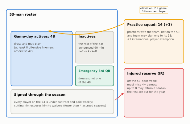
The roster is big and the game is specialized. A team carries 53 players, dresses 48 on game day, and needs starters at about 25 different jobs once you count the kicker, punter and long snapper. A left tackle can’t play cornerback. So the budget can’t simply follow “buy the best players”; it has to buy a team, with a backup at every spot the season will expose.

Most talent arrives through a draft you don’t control. The worst teams pick first, and rookies are paid on a fixed scale. That makes the draft the cheapest source of good players, and it means a team’s cost of talent depends on when it acquired a player as much as on how good he is.

Put those together and the GM’s real question isn’t “who is good?” It is “where does the next dollar, or the next pick, buy the most winning?” The rest of this chapter is the toolkit for answering it.

ImportantWhy it exists: the salary cap

The cap is a deal between the owners and the players’ union, renewed in each collective bargaining agreement (the current one, signed in 2020, runs through the 2030 season). The players get a fixed share of league revenue, at least 48 percent, paid out through the cap and benefits; the owners get cost certainty and a league in which a small-market team can afford the same roster as a big-market one.² The trade-off is the one this chapter keeps returning to: under a hard cap, overpaying anyone is never free, because someone else on the roster pays for it.

NoteMadden vs. real life

In Madden’s franchise mode, cutting an expensive veteran usually frees his whole salary. In the NFL, a release can cost cap space this year, because of the bonus money already paid (the dead money section below shows why). And no real GM can trade three backups for a star the way the game’s AI often accepts: picks and players are priced by charts every front office knows.

Positional value: not every position is worth the same

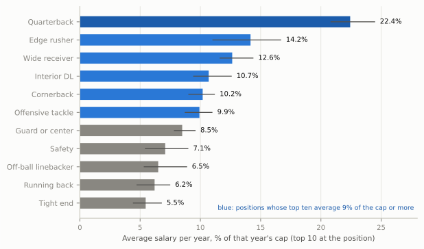
Start with what teams actually pay. Figure 72.1 shows the ten richest active contracts at each position, measured the way cap analysts compare deals across years: average salary per year (APY, the contract’s total value divided by its years) as a share of the salary cap in the year the deal was signed.

fig, ax = plt.subplots(figsize=(6.5, 3.9))
order = TOP10.index.tolist()
y = np.arange(len(order))
cols = [style.OFFENSE_DARK if g == "Quarterback" else (style.OFFENSE if m >= 0.09 else style.MUTED)
        for g, m in zip(order, TOP10["mean"])]
ax.barh(y, 100 * TOP10["mean"], color=cols, height=0.62, zorder=2)
ax.hlines(y, 100 * TOP10["min"], 100 * TOP10["max"], color=style.INK_2, lw=1.0, zorder=3)
for yi, (g, r) in zip(y, TOP10.iterrows()):
    ax.text(100 * r["max"] + 0.4, yi, f"{100 * r['mean']:.1f}%", va="center", fontsize=7.5, color=style.INK)
ax.set_yticks(y)
ax.set_yticklabels(order, fontsize=8)
ax.set_xlabel("Average salary per year, % of that year's cap (top 10 at the position)", fontsize=8)
ax.set_xlim(0, 100 * TOP10["max"].max() + 3.5)
ax.grid(axis="y", visible=False)
ax.tick_params(axis="x", labelsize=7.5)
ax.text(0.99, 0.04, "blue: positions whose top ten average 9% of the cap or more", transform=ax.transAxes,
        ha="right", fontsize=7.0, color=style.OFFENSE_DARK)
fig.tight_layout()
plt.show()

Figure 72.1: The market’s verdict on positional value. Each bar is the average of the ten richest active contracts at that position as of the 2026 season, measured as average salary per year (APY) divided by the salary cap in the year the contract was signed; the thin line runs from the tenth-richest to the richest deal. Left and right tackles are counted together. A top-ten quarterback is paid about one and a half times what a top-ten edge rusher is and more than three times what a top-ten running back is. Data: Over the Cap contract data via nflverse (load_contracts).

That chart is positional value as the market sees it: how much a position, not a particular player, contributes to winning, and so how much it’s worth paying for. Quarterback is alone at the top, at 22.4% of the cap for a top-ten deal. Then come the premium positions: edge rusher and wide receiver, then a cluster of interior defensive linemen, offensive tackles and cornerbacks at about 9 to 11 percent. Below them come guards and centers at about 8.5 percent, then safeties, off-ball linebackers, running backs and tight ends at roughly 5.5 to 7 percent. (Interior defensive line is high because the market pays a few rare interior pass rushers like edge rushers; a run-stuffing tackle is paid far less.) Each step has a reason.

Quarterback touches every snap. He decides where the ball goes on every pass and many runs, and Expected Points showed that passing plays carry more value per snap than runs and swing far more widely. A position that controls the highest-leverage action on every play is worth more than one that matters on a third of them.

The premium group decides the passing game. An edge rusher who wins one-on-one ends drives with sacks and hurried throws; the offensive tackles are the men assigned to stop him. The old idea was that only the left tackle mattered, because he guards a right-handed quarterback’s blind side, the side he can’t see. The market no longer believes it: 4 of the ten richest tackle contracts belong to right tackles. A receiver who wins against man coverage gives the quarterback somewhere to throw; and a cornerback who can cover him alone frees the rest of the defense to help elsewhere. Every one of those players wins or loses a matchup on most passing downs, and they are scarce: you can’t develop a 6-foot-5, 265-pound man who runs a 4.5 forty from the seventh round.

The bottom group is either replaceable or rarely decisive. Running back is the classic case. Most of a run’s yards are created by the blockers and the scheme before the back touches the ball (13-02’s rush-yards-over-expected showed how little separates most backs once you account for the blocking), backs wear down quickly, and the college game produces good ones every year. Off-ball linebackers and safeties matter, but they win fewer one-on-one matchups that decide plays, and they are easier to find.

CautionCommon misconception

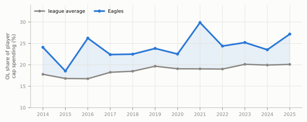
“Running backs don’t matter.” Positional value is about price, not about whether a position matters. Saquon Barkley ran for 2,005 yards for the 2024 Eagles and was central to a Super Bowl run (the Eagles case study tells it). The argument is narrower: the gap between a great back and a decent one is smaller than the gap between their salaries, so the money usually buys more at another position. The Eagles could pay Barkley because they had built cheaply elsewhere, which is the real lesson of positional value.

Does spending on a position buy wins?

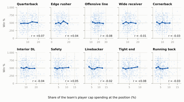
If some positions are worth more, you might expect teams that spend more of their cap on them to win more. Figure 72.2 tests that directly, for every team-season from 2014 to 2025: how much of its player spending went to each position group, against its winning percentage.

groups = ["QB", "EDGE", "OL", "WR", "CB", "IDL", "S", "LB", "TE", "RB"]
fig, axes = plt.subplots(2, 5, figsize=(6.6, 3.6), sharey=True)
for ax, g in zip(axes.flat, groups):
    x = 100 * TEAMS[g]
    ax.scatter(x, TEAMS.winpct, s=3, color=style.OFFENSE, alpha=0.18, lw=0, zorder=2)
    q = pd.qcut(x, 5)
    m = TEAMS.groupby(q, observed=True).winpct.mean()
    xm = x.groupby(q, observed=True).mean()
    ax.plot(xm, m, color=style.OFFENSE_DARK, lw=1.8, marker="o", ms=2.6, zorder=3)
    ax.axhline(0.5, color=style.BASELINE, lw=0.7, zorder=1)
    ax.set_title(GROUP_NAME[g], fontsize=7.6, loc="left")
    ax.text(0.97, 0.05, f"r = {R_BY_GROUP[g]:+.2f}", transform=ax.transAxes, ha="right", fontsize=6.8,
            color=style.INK)
    ax.tick_params(labelsize=6.2)
    ax.set_ylim(0, 1)
    ax.set_yticks([0, 0.25, 0.5, 0.75, 1.0])
for ax in axes[:, 0]:
    ax.set_yticklabels(["0", ".250", ".500", ".750", "1.000"])
    ax.set_ylabel("Win %", fontsize=7)
fig.supxlabel("Share of the team's player cap spending at the position (%)", fontsize=7.5)
fig.tight_layout()
plt.show()

Figure 72.2: Positional cap share against winning, every team-season 2014–2025. Each faint dot is one team-season: the share of the team’s player cap spending that went to that position group (x) and its regular-season winning percentage (y). The dark line joins the average winning percentage in each fifth of the spending range; r is the correlation. Every line is close to flat: how much a team spent on a position, quarterback included, says almost nothing about how often it won. Dead money is not included, so shares are of money spent on players on the roster. Data: Over the Cap contract histories via nflverse; nflverse schedules.

Every line is close to flat. Across 384 team-seasons, the correlation between a position group’s share of spending and winning is never stronger than 0.08 in either direction, and for quarterbacks it is +0.07. Does that mean positional value is a myth? No. It means price and value are different things, for three reasons.

1. The cap is zero-sum. Spending 20 percent of the cap on a quarterback means spending 20 percent less on everyone else. A team that pays one star well and fills the rest with bargains can end up anywhere.
2. Contracts pay for the past. Teams sign big deals with players who were great, and pay them through their late twenties and early thirties, when many decline. A big share can be a reward for seasons already played.
3. The best bargains are on rookie contracts. The cheapest good players in the league are young ones on the rookie wage scale, which is the subject of the draft section. A team with a great young quarterback spends less on the position than a team overpaying a mediocre veteran.

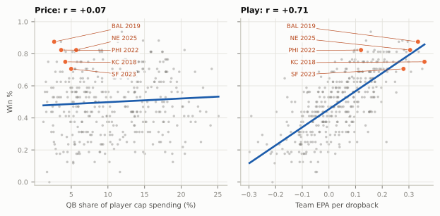
The quarterback case makes the point clearest. Figure 72.3 sets the price of the position against the quality of the play.

fig, (a1, a2) = plt.subplots(1, 2, figsize=(6.6, 3.3), sharey=True)
a1.scatter(100 * TEAMS.QB, TEAMS.winpct, s=7, color=style.MUTED, alpha=0.45, lw=0)
a2.scatter(TEAMS.db_epa, TEAMS.winpct, s=7, color=style.MUTED, alpha=0.45, lw=0)
for ax, xcol, scale in ((a1, "QB", 100), (a2, "db_epa", 1)):
    xx = scale * TEAMS[xcol]
    b, c = np.polyfit(xx, TEAMS.winpct, 1)
    xs = np.linspace(xx.min(), xx.max(), 10)
    ax.plot(xs, b * xs + c, color=style.OFFENSE_DARK, lw=2)
    ax.tick_params(labelsize=7)
    ax.set_ylim(-0.02, 1.02)
cheap = [((2019, "BAL"), "BAL 2019"), ((2025, "NE"), "NE 2025"), ((2022, "PHI"), "PHI 2022"),
         ((2018, "KC"), "KC 2018"), ((2023, "SF"), "SF 2023")]
cheap = sorted(cheap, key=lambda kv: -TEAMS.loc[kv[0]].winpct)       # top-down, so leader lines don't cross
for i, (key, lab) in enumerate(cheap):
    r = TEAMS.loc[key]
    ly = 0.97 - 0.075 * i
    for ax, xv, lx, ha in ((a1, 100 * r.QB, 10.5, "left"), (a2, r.db_epa, -0.05, "right")):
        ax.scatter([xv], [r.winpct], s=26, color=style.SERIES[1], zorder=4, edgecolor="white", lw=0.6)
        ax.annotate(lab, (xv, r.winpct), (lx, ly), fontsize=6.4, color=style.DEFENSE_DARK, ha=ha, va="center",
                    zorder=5, bbox=dict(boxstyle="round,pad=0.15", fc=style.SURFACE, ec="none", alpha=0.9),
                    arrowprops=dict(arrowstyle="-", color=style.DEFENSE_DARK, lw=0.5, shrinkA=0, shrinkB=3))
a1.set_xlabel("QB share of player cap spending (%)", fontsize=7.5)
a2.set_xlabel("Team EPA per dropback", fontsize=7.5)
a1.set_ylabel("Win %", fontsize=7.5)
a1.set_title(f"Price: r = {R_QB_PRICE:+.2f}", fontsize=8.5)
a2.set_title(f"Play: r = {R_QB_PLAY:+.2f}", fontsize=8.5)
fig.tight_layout()
plt.show()

Figure 72.3: Price versus play at quarterback, every team-season 2014–2025. Left: the share of the team’s player cap spending that went to quarterbacks against winning percentage. It is close to flat. Right: the team’s EPA per dropback (every pass attempt, sack and scramble) against winning percentage. It is steep. The labelled seasons are teams whose starting quarterback was on a rookie contract (Mahomes in 2018, Jackson in 2019, Hurts in 2022, Purdy in 2023, Maye in 2025): elite play, low price, the most valuable combination in the sport. Data: Over the Cap via nflverse; nflverse play-by-play and schedules.

How well a team passes correlates with winning at 0.71, about as strong as anything in football statistics; how much it pays its quarterbacks correlates at 0.07. (EPA per dropback isn’t only the quarterback, of course: the line and receivers are in it too. But the quarterback is the largest single piece.) The value is in the play. The money is a separate question, and the gap between the two is where rosters are won. The labelled seasons show the best gap there is: a quarterback playing like a star on a rookie salary. Each of those teams used the savings to buy help; four of the five reached at least a conference championship game, and three reached the Super Bowl.

That is the whole logic of roster building in miniature. Pay for value where you must, and get value cheaply wherever you can. The tools for “cheaply” are the draft and the cap rules, and the next sections take them one at a time.

How a contract really hits the cap

A headline says “five years, $150 million.” Almost none of that number tells you what the team will actually carry on its cap in a given year, or what it would cost to get out of the deal. Four ideas do.

The cap hit is what a contract counts against the cap in one league year: the player’s base salary for that year, plus the year’s share of his signing bonus, plus any roster, workout or incentive bonuses counted that year. It is an accounting number, not the cash paid. The broadcast graphic shows it because it’s the number that limits the team.

Signing-bonus proration is the rule that creates the gap between cash and cap. A signing bonus is paid to the player up front (often within months), but for cap purposes it is spread evenly over the years of the contract, up to a maximum of five. That is why teams love signing bonuses: the player gets the cash now, and the team spreads the cap cost into future years, when the cap will usually be higher, so the same fixed charge is a smaller share of it.

Guaranteed money is money the team must pay even if it releases the player. It comes in flavors: fully guaranteed at signing (owed no matter what), injury-only (owed if he is cut while hurt), and money that vests, becoming fully guaranteed on a set date, often a few days into the new league year, if he is still on the roster. Agents and reporters often quote the total of all of these, which is why “total guarantees” in a headline can be far larger than what the player is truly certain to receive.

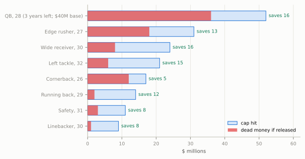
Dead money is the bill for leaving early. If a team releases or trades a player, every year of signing-bonus proration not yet counted lands on the cap at once, along with any guaranteed salary still owed. That money pays for nobody on the field.

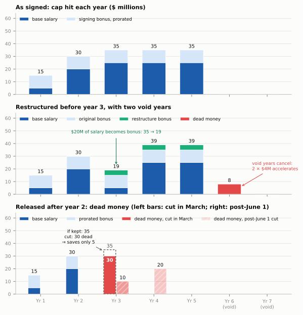
Figure 72.4 walks one invented contract through all of it.

YEARS = ["Yr 1", "Yr 2", "Yr 3", "Yr 4", "Yr 5", "Yr 6\n(void)", "Yr 7\n(void)"]
BASE = np.array([5, 20, 25, 25, 25, 0, 0], float)
PRO = np.array([10, 10, 10, 10, 10, 0, 0], float)
fig, axes = plt.subplots(3, 1, figsize=(6.5, 6.6), sharex=True)
x = np.arange(7)


def stack(ax, layers, totals=True, dx=0.0, width=0.62):
    bottom = np.zeros(7)
    for vals, color, lab in layers:
        ax.bar(x + dx, vals, width, bottom=bottom, color=color, label=lab, zorder=2, edgecolor="white", lw=0.5)
        bottom += vals
    if totals:
        for xi, t in zip(x, bottom):
            if t > 0:
                ax.text(xi + dx, t + 0.8, f"{t:.0f}", ha="center", va="bottom", fontsize=7.2, color=style.INK)
    return bottom


ax = axes[0]
stack(ax, [(BASE, style.OFFENSE_DARK, "base salary"), (PRO, style.OFFENSE_TINT, "signing bonus, prorated")])
ax.set_title("As signed: cap hit each year ($ millions)", fontsize=8.5)
ax.legend(fontsize=6.6, loc="upper left", ncol=4)

ax = axes[1]
b2 = BASE.copy(); b2[2] = 5
new = np.array([0, 0, 4, 4, 4, 0, 0], float)
dead_void = np.array([0, 0, 0, 0, 0, 8, 0], float)
stack(ax, [(b2, style.OFFENSE_DARK, "base salary"), (PRO, style.OFFENSE_TINT, "original bonus"),
           (new, style.THIRD, "restructure bonus"), (dead_void, RED, "dead money")])
ax.annotate("$20M of salary becomes bonus: 35 → 19", (2.0, 22.5), (2.0, 49), fontsize=6.6, color=GREEN,
            ha="center", va="center", arrowprops=dict(arrowstyle="->", color=GREEN, lw=0.8, shrinkA=4))
ax.annotate("void years cancel:\n2 × $4M accelerates", (5.3, 6), (5.6, 22), fontsize=6.6, color=RED, ha="left",
            va="center", arrowprops=dict(arrowstyle="->", color=RED, lw=0.8))
ax.set_title("Restructured before year 3, with two void years", fontsize=8.5)
ax.legend(fontsize=6.6, loc="upper left", ncol=4)

ax = axes[2]
pre = [(np.array([5, 20, 0, 0, 0, 0, 0], float), style.OFFENSE_DARK, "base salary"),
       (np.array([10, 10, 0, 0, 0, 0, 0], float), style.OFFENSE_TINT, "prorated bonus"),
       (np.array([0, 0, 30, 0, 0, 0, 0], float), RED, "dead money, cut in March")]
post_dead = np.array([0, 0, 10, 20, 0, 0, 0], float)
stack(ax, pre, totals=False, dx=-0.17, width=0.32)
for xi, t in ((0, 15), (1, 30)):
    ax.text(xi - 0.17, t + 0.8, f"{t}", ha="center", va="bottom", fontsize=7.2, color=style.INK)
ax.text(2 - 0.17, 26.5, "30", ha="center", va="center", fontsize=7.2, color="white", fontweight="bold", zorder=5)
ax.text(2 - 0.17, 35.8, "35", ha="center", va="bottom", fontsize=7.2, color=style.INK_2)
ax.bar(x[2:4] + 0.17, post_dead[2:4], 0.32, color=RED, alpha=0.55, zorder=2, edgecolor="white", lw=0.5,
       hatch="///", label="dead money, post-June 1 cut")
for xi, v in zip(x[2:4], post_dead[2:4]):
    ax.text(xi + 0.17, v + 0.8, f"{v:.0f}", ha="center", va="bottom", fontsize=7.2, color=style.INK)
# ghost of the year-3 cap hit as signed, so "saves only 5" can be seen: 35 if kept, 30 if cut in March
ax.bar(x[2] - 0.17, 35, 0.32, fill=False, edgecolor=style.INK_2, lw=0.9, ls=(0, (3, 2)), zorder=4)
ax.annotate("if kept: 35\ncut: 30 dead\n→ saves only 5", (x[2] - 0.34, 34), (1.0, 45), fontsize=6.6,
            color=style.INK, ha="center", va="center",
            arrowprops=dict(arrowstyle="->", color=style.INK_2, lw=0.7))
ax.set_title("Released after year 2: dead money (left bars: cut in March; right: post-June 1)", fontsize=8.5)
ax.legend(fontsize=6.6, loc="upper left", ncol=4)
for ax in axes:
    ax.set_ylim(0, 64)
    ax.tick_params(labelsize=7)
    ax.grid(axis="x", visible=False)
axes[2].set_xticks(x)
axes[2].set_xticklabels(YEARS, fontsize=7)
fig.tight_layout()
plt.show()

Figure 72.4: One invented contract, three ways. Five years, $150 million: a $50 million signing bonus and base salaries of $5, 20, 25, 25 and 25 million. Top: as signed, the bonus counts $10 million a year (light blue) on top of each year’s base salary (dark blue); the cap hits are 15, 30, 35, 35 and 35. Middle: before year 3 the team restructures, turning $20 million of that year’s salary into a new bonus and spreading it over the three real years left plus two void years (aqua, $4 million a year). Year 3’s cap hit falls from 35 to 19, but years 4 and 5 rise, and when the void years cancel, their $8 million lands as dead money (red). Bottom: the team cuts the player after year 2 instead. Before June 1, all $30 million of unspent bonus becomes dead money in year 3; against the $35 million he would have counted if kept (dashed outline), that saves only $5 million of cap; with a post-June 1 designation the dead money is split, $10 million in year 3 and $20 million in year 4.

Read the top panel first. The player is paid $55 million in cash in year 1 (the $50 million bonus plus $5 million of salary), but the team counts only $15 million against the cap. That gap is why every big contract is built around a large signing bonus: it front-loads the player’s money and back-loads the team’s cap cost. Typically the bonus plus the first year or two of salary are fully guaranteed at signing, here $75 million, and the later years are not, which is what makes them “team-friendly”: the team can walk away from them.

Restructures and void years: borrowing from the future

The middle panel is the most common move in the cap world, the restructure. A team needs cap space this year, so it asks a player it plans to keep to turn most of this year’s base salary into a signing bonus. The player loses nothing: he gets the same money sooner, it becomes guaranteed, and the extra dead money it creates makes him harder to cut, which is job security. The team spreads the new bonus over the remaining years and cuts this year’s cap hit sharply. The catch is that later cap hits rise by the same total, so a restructure is borrowing, not saving.

Void years stretch the loan. They are fake final years added to the contract that cancel automatically before anyone plays them. Their only purpose is to give the bonus more years to spread across, which lowers each year’s charge. When they cancel, whatever proration was assigned to them becomes dead money all at once. The league tolerates them because they move cap charges without erasing any: every bonus dollar still counts against some year’s cap. Tom Brady’s last Tampa Bay contracts were the famous example: after he retired in February 2023, the Buccaneers carried about $35 million of dead money for a quarterback who was no longer playing.³

Cutting a player, and why June 1 matters

The bottom panel is the release. After year 2, the player’s last three years carry $30 million of proration that hasn’t been counted. Cut him in March and all $30 million is dead money this year, so the release saves only $5 million of cap (his $35 million cap hit minus $30 million of dead money) even though it saves $25 million of cash. That is why you hear “they can’t afford to cut him”: sometimes cutting a player costs nearly as much cap space as keeping him.

The June 1 rule softens it. If a player is released after June 1, or released earlier with a post-June 1 designation (each team gets two a year), only the current year’s proration counts this year and the rest moves to next year. The team gets more room now and pays the remainder later. The catch is timing: a designated player’s full cap hit stays on the books until June 2, so the designation doesn’t help a team that needs room in March, when free agency opens.

Two more rules shape how much room a team really has. From the start of the league year until the season, only a team’s 51 largest contracts count in full (the top-51 rule), so cutting a player saves his cap hit minus the cost of the minimum-salary player who moves up into the top 51. And unused cap space can be carried over into the next league year, which is why some teams deliberately “bank” room.⁴

NoteFilm room: Denver Broncos, 2024

The move: Denver released quarterback Russell Wilson two years after trading for him and signing him to a five-year, $245 million extension. The release created $85 million of dead money, the largest amount in league history at the time.⁵

Why March: on the fifth day of the 2024 league year, another $37 million of Wilson’s future salary would have turned from guaranteed-for-injury into fully guaranteed. Cutting him on the first day of the league year kept that money off the bill. Why two years: the release carried a post-June 1 designation, so the charge was split across two league years, and Denver chose to take the larger part, a record $53 million, on the 2024 cap and $32 million on 2025.

What to notice: why a team would accept that. Wilson’s remaining guaranteed money had to be paid either way, so keeping him cost the same money plus a roster spot for a player the coaches had benched. Dead money is a sunk cost: it is spent whatever you do next, and good front offices decide on what each choice costs from here. Denver spent 2024 with a rookie quarterback, Bo Nix, on a rookie contract, and made the playoffs; in 2025 it went 14–3 and earned the AFC’s top seed while still carrying the second half of the Wilson charge. A painful cap year is survivable when the replacement is cheap.

Getting players: free agency, tags, trades and waivers

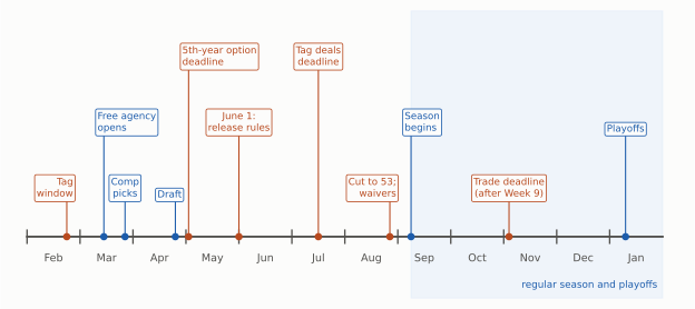
Every route onto a roster has a price, and the price is paid in different currencies: cap space, draft picks, or the right to a player in future years. Figure 72.5 puts the routes on the calendar, because when each one is open shapes how teams use it.

EVENTS = [  # (position: 0 = Feb 1, 1 = Mar 1, ...; label; row; kind; label alignment)
    (0.75, "Tag\nwindow", 0, "dead", "right"),
    (1.45, "Free agency\nopens", 1, "acq", "left"),
    (1.85, "Comp\npicks", 0, "acq", "center"),
    (2.8, "Draft", 0, "acq", "right"),
    (3.05, "5th-year option\ndeadline", 2, "dead", "left"),
    (4.0, "June 1:\nrelease rules", 1, "dead", "center"),
    (5.5, "Tag deals\ndeadline", 2, "dead", "center"),
    (6.85, "Cut to 53;\nwaivers", 0, "dead", "right"),
    (7.25, "Season\nbegins", 1, "acq", "left"),
    (9.1, "Trade deadline\n(after Week 9)", 0, "dead", "center"),
    (11.3, "Playoffs", 1, "acq", "center"),
]
MONTHS = ["Feb", "Mar", "Apr", "May", "Jun", "Jul", "Aug", "Sep", "Oct", "Nov", "Dec", "Jan"]
fig, ax = plt.subplots(figsize=(6.6, 3.0))
ax.plot([0, 12], [0, 0], color=style.INK_2, lw=1.4, zorder=1)
for i, m in enumerate(MONTHS):
    ax.plot([i, i], [-0.08, 0.08], color=style.INK_2, lw=1)
    ax.text(i + 0.5, -0.3, m, ha="center", fontsize=7.2, color=style.INK_2)
ax.axvspan(7.25, 12, ymin=0.0, ymax=1.0, color=style.OFFENSE_TINT, alpha=0.35, zorder=0)
ax.text(11.9, -0.62, "regular season and playoffs", ha="right", fontsize=6.6, color=style.OFFENSE_DARK)
for xpos, lab, row, kind, ha in EVENTS:
    yy = 0.45 + 0.8 * row
    c = style.OFFENSE_DARK if kind == "acq" else style.DEFENSE_DARK
    ax.plot([xpos, xpos], [0, yy], color=c, lw=0.8, zorder=2)
    ax.scatter([xpos], [0], s=16, color=c, zorder=3)
    lx = xpos + {"left": -0.12, "right": 0.12, "center": 0.0}[ha]
    ax.text(lx, yy, lab, ha=ha, va="bottom", fontsize=6.5, color=c, zorder=4,
            bbox=dict(boxstyle="round,pad=0.2", fc=style.SURFACE, ec=c, lw=0.6))
ax.set_xlim(-0.3, 12.4)
ax.set_ylim(-0.75, 2.75)
ax.axis("off")
fig.tight_layout()
plt.show()

Figure 72.5: The NFL’s business calendar (approximate dates; exact days shift each year). The league year turns over in mid-March, when contracts expire, free agency opens, and trades agreed since the end of the season can finally be processed. Tags are placed in the two weeks before, and a tagged player has until mid-July to sign a long-term deal; compensatory picks are awarded in March; the draft comes in late April and fifth-year options are due in early May; the June 1 date changes how releases count; rosters are cut to 53 in late August; the trade deadline falls in early November, after Week 9; and waivers run all year. Blue: acquiring players; orange: deadlines and cuts.

Free agency: unrestricted and restricted

When a contract expires, what happens depends on the player’s accrued seasons, the seasons in which he spent at least six regular-season games on full pay status (on the active roster, inactive, or on injured reserve).

• An unrestricted free agent (UFA) has four or more accrued seasons. He may sign with anyone, and his old team gets nothing back except possibly a compensatory pick a year later (explained below). This is the market most fans picture: the first days of the league year in March, when the best players sign big deals, usually agreed during a two-day negotiating window just before it that broadcasters call “legal tampering”.
• A restricted free agent (RFA) has exactly three. His team can offer him a one-year tender at one of several set prices. He may then sign an offer sheet with another team, but his old team can match it; if it doesn’t, it receives a draft pick whose round depends on the tender. Offer sheets are rare, because teams don’t like giving up picks to pry a player loose. (With fewer than three seasons, a player can be kept for a minimum salary and can’t negotiate elsewhere at all.)

Why free agency exists: it is the players’ half of the 1993 bargain that also created the cap (see 11-02). What it costs teams: free agents are usually paid for what they did on their last team, at the peak of their market, and a bidding war means the team that “wins” is the one that valued him most, often too much. Analysts call that the winner’s curse, and it’s why patient teams treat free agency as a way to fill specific holes rather than to build a roster.

The franchise and transition tags

What if the player is a star and the team can’t agree on a long-term deal? It can tag him.

The franchise tag is a one-year contract that a team may impose on one expiring player a year. Its price is set by formula: roughly the average of the five largest cap numbers at his position, or 120 percent of his previous salary, whichever is higher. The usual non-exclusive tag lets other teams bid, but his team may match, and if it doesn’t it receives two first-round picks, a price that almost always ends the conversation; the pricier exclusive tag forbids talking to other teams at all.

The transition tag is the cheaper version, priced from the top ten salaries at the position. Other teams can sign the player to an offer sheet, and his team gets only the right to match, with no compensation if it lets him go.⁶

Why tags exist: to let a team keep a great player for one more season while the two sides keep negotiating; a tagged player and his team have until mid-July to agree on a long-term deal, or he plays the year on the tag. What a tag costs: a full year of top-of-market salary, fully guaranteed, with no cap-friendly bonus structure, and a player who usually feels he has been denied his long-term security. Tagging the same player again costs more each time. Washington tagged quarterback Kirk Cousins in 2016 and again in 2017, then let him walk; Minnesota signed him in 2018 to a three-year, $84 million contract that was fully guaranteed, the first multi-year fully guaranteed deal for a quarterback and a direct result of the leverage two tags had given him.⁷

Because the tag is priced by position, it is also where scheme meets money. In 2014 the Saints tagged Jimmy Graham as a tight end, at about $7 million; Graham argued that he lined up in the slot or out wide so often that he was really a receiver, whose tag was about $12.3 million. An arbitrator ruled that a tight end detached from the line in the slot is still doing a tight end’s job, and Graham lost.⁸ The label on a player’s role is worth millions, which is the idea Scheme and Fantasy picks up.

Compensatory picks

A team that loses more good free agents than it signs gets a consolation prize. The compensatory pick formula looks at every unrestricted free agent who left or arrived the previous year, ranks each by his new contract’s average salary, playing time and honors, and awards up to 32 extra picks league-wide, at the end of rounds 3 through 7, at most four per team. Since 2017 the picks can be traded.⁹ The idea is to repay a team for talent it developed and then lost on the open market.

Why it matters for strategy: the formula nets the two lists. Every qualifying free agent a team signs cancels out one it lost, roughly matched by contract size. Only players whose contracts ran out count; a player who was released doesn’t count on either side. So a team can choose to let its own free agents walk, sign only veterans other teams have cut, and collect the picks.¹⁰ The Baltimore Ravens are the model: they have received more compensatory picks than any other franchise since the system began in 1994, and their roster is built on letting expensive veterans walk at the right time.¹¹

Trades and the trade deadline

A trade moves a contract, not just a player. The acquiring team takes over his remaining salary and cap hits; the trading team keeps any signing-bonus proration it has not yet counted, as dead money. When a broadcast says a team “ate” money to make a deal work, that is what it means: it took a dead-money charge so that the other team would take the player. Trades also cluster around the new league year in March, because a trade agreed after the season can’t be processed until then, and because that is when next year’s cap numbers start to count.

The trade deadline is the last day of the season on which trades are allowed: since 2024, the Tuesday after Week 9.¹² After it, a contender can add only free agents, waiver claims and its own practice squad. So contenders use the deadline to rent a veteran for a playoff run, paying with future picks, and sellers turn a player who won’t be part of their next good team into a pick that might be.

Waivers

When a team releases a player with fewer than four accrued seasons (and, after the trade deadline, any player, so that a contender can’t sign a veteran whom a rival releases to get around the deadline), he goes on waivers: for about a day, every other team may claim him and take over his contract as it stands. If several teams claim him, the one with the worst record wins. A player nobody claims becomes a free agent and can choose his next team. Waivers matter most on cut-down day in late August, when hundreds of players are released at once and every front office combs the list for someone better than its own 53rd man.

NoteFilm room: Los Angeles Rams, 2021

The build: the Rams of 2021 are the boldest trade-built champion of the cap era. In March they made official the trade for quarterback Matthew Stafford, sending Detroit Jared Goff, a 2021 third-round pick and their first-round picks in 2022 and 2023. They already had cornerback Jalen Ramsey, acquired in 2019 for two first-round picks and a fourth. At the trade deadline they added edge rusher Von Miller for a 2022 second- and third-round pick. A week later Cleveland released Odell Beckham Jr. Because the deadline had passed, even a veteran had to go through waivers; nobody claimed his contract, which made him a free agent free to pick his team, and he chose Los Angeles.¹³ On February 13, 2022, the Rams beat Cincinnati 23–20 in Super Bowl LVI: Beckham caught the game’s first touchdown, Miller had two sacks, and Stafford threw three touchdown passes.

What to notice: the currency. The Rams paid in future draft picks, which a team with a short window values least, and spent them on premium positions (a quarterback, a cornerback, an edge rusher) rather than on depth. The bill came later: the Rams did not make a first-round pick in any draft from 2017 through 2023 (their first after Jared Goff in 2016 was Jared Verse, 19th overall in 2024), and went 5–12 in 2022 with an injured, expensive roster. They drafted their way back (Puka Nacua was a 2023 fifth-round pick) and were back in the playoffs in 2023. A trade-built roster wins a window; it doesn’t build a pipeline.

The draft: the cheapest good players in football

The rookie wage scale and the fifth-year option

Before 2011, top draft picks negotiated like free agents, and the price had run away: the 2010 first overall pick, quarterback Sam Bradford, signed a six-year deal worth up to $78 million with $50 million guaranteed before playing a down, more than many proven veteran quarterbacks earned. The 2011 collective bargaining agreement ended that with the rookie wage scale. Every draft slot now carries a set four-year contract value, falling steeply from the first pick to the last, with little left to negotiate. Drafted players cannot sign an extension until after their third regular season.¹⁴

First-round picks come with one extra year of team control. The fifth-year option lets the team add a fifth season at a set price, decided after the player’s third season (by early May). Since the 2020 agreement the option is fully guaranteed once exercised, and its price depends on how much the player has played and whether he made Pro Bowls, so teams now decline it for players they aren’t sure of.

Together these rules create the rookie-contract window: the years in which a good young player is paid far less than a veteran of his quality. For a star it usually lasts three seasons, not four or five, because the first moment an extension is allowed (after year 3) is also the moment his team rushes to lock him up before his price climbs further. For most positions the window is a nice bonus. For a quarterback it is the most valuable asset in the sport, as Figure 72.3 showed, and teams with a young starter build their entire cap plan around it.

Draft value charts: what is a pick worth?

To trade picks, teams need a common price list. The original draft value chart was built for the Dallas Cowboys in the early 1990s, under head coach Jimmy Johnson, from past trades and judgment: at Johnson’s request, Cowboys vice president Mike McCoy drew it up before the club’s run of draft-day trades in 1991.¹⁵ The Jimmy Johnson chart gives the first pick 3,000 points, the 16th 1,000, the 32nd 590, the 64th 270 and the 100th 100. Teams still use it or close cousins, and a trade that “balances on the chart” is still how deals get done. (Separately, each team ranks the prospects themselves on its draft board, its own ordered list of players; the chart prices the slots, the board decides whom to take in them.)

But the chart describes what teams pay for picks, not what the picks produce. In 2005 two behavioral economists, Cade Massey and Richard Thaler (Thaler later won a Nobel prize for work on how people make predictable mistakes), asked whether the prices were right. They measured each pick’s surplus value: what a player produces minus what he is paid. Their answer, published as “The Loser’s Curse,” was that teams badly overvalue the top of the draft. A top pick is more likely to become a star, but he is also paid far more, and teams are overconfident in their ability to tell the stars apart. By surplus value, they found, picks gained value through the first round, because a pick’s cost fell faster down the round than the production teams could expect from it, and the best value in the draft sat in the second round.¹⁶ The curse of the title: the worst team earns the first pick, and the first pick is overpriced.

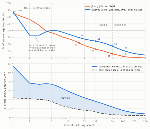
Their data came from before the rookie wage scale, when top picks were far more expensive. We can redo the idea for the current era with contract data. For every player drafted from 2011 to 2020, take what the market paid him on his next contract (as a share of the cap) as the measure of what he turned out to be worth, and take his rookie salary as what he cost. Surplus is the difference. Why the next contract? Because when a rookie deal ends, 32 front offices that watched him for four years bid on him, and the price they settle on is the best available summary of how good he was; a player nobody would pay counts as zero. The two halves come from different years on purpose: value from the 2011–2020 classes, because later classes haven’t all reached a second contract yet, and cost from 2021–2025 rookie deals, because those are today’s prices. Figure 72.6 compares that curve with the Johnson chart.

fig, (a1, a2) = plt.subplots(2, 1, figsize=(6.5, 5.6), sharex=True)
a1.plot(PICKS, 100 * JJ / JJ_TOP10, color=style.SERIES[1], lw=2.2, label="Jimmy Johnson chart")
a1.plot(PICKS, 100 * SURPLUS / SV_TOP10, color=style.OFFENSE, lw=2.4,
        label="Surplus value (contracts, 2011–2020 classes)")
a1.axhline(100, color=style.BASELINE, lw=0.8, zorder=0)
for pk in (32.5, 64.5):
    a1.axvline(pk, color=style.BASELINE, lw=0.8, ls=(0, (3, 3)), zorder=0)
for pk in (16, 32, 64, 100):
    a1.scatter([pk], [jj_rel(pk)], s=14, color=style.SERIES[1], zorder=4)
    a1.scatter([pk], [sv_rel(pk)], s=14, color=style.OFFENSE, zorder=4)
    if pk < 100:     # below-left of a falling curve sits clear of the line
        a1.text(pk * 0.93, jj_rel(pk) - 4, f"{jj_rel(pk):.0f}", fontsize=6.8, color=style.DEFENSE_DARK,
                ha="right", va="top")
    else:            # near the floor: above-right instead, so it stays off the x-axis
        a1.text(pk * 1.07, jj_rel(pk) + 5, f"{jj_rel(pk):.0f}", fontsize=6.8, color=style.DEFENSE_DARK)
    a1.text(pk * 1.07, sv_rel(pk) + 5, f"{sv_rel(pk):.0f}", fontsize=6.8, color=style.OFFENSE_DARK)
a1.annotate(f"picks 2–3: only {N23} players,\n{N23_BUST} were paid less on their\nnext deal than as rookies",
            (2.5, sv_rel(2.5) - 2), (3.4, 36), fontsize=6.3, color=style.INK_2, ha="center", va="center",
            arrowprops=dict(arrowstyle="-", color=style.INK_2, lw=0.6))
a1.annotate(f"No. 1: {N1_QB} of 10 were QBs", (1.0, sv_rel(1)), (1.6, 182), fontsize=6.6, color=style.INK_2,
            va="center", arrowprops=dict(arrowstyle="-", color=style.INK_2, lw=0.6))
a1.set_ylabel("% of an average top-10 pick", fontsize=8)
a1.set_ylim(0, 200)
a1.legend(fontsize=7, loc="upper right")
a1.text(36, 118, "round 2", fontsize=6.6, color=style.INK_2)
a1.text(70, 118, "round 3 on", fontsize=6.6, color=style.INK_2)
a2.fill_between(PICKS, 100 * COST, 100 * VALUE, where=VALUE > COST, color=style.OFFENSE, alpha=0.15, lw=0)
a2.plot(PICKS, 100 * VALUE, color=style.OFFENSE, lw=2.2, label="value: next contract, % of cap per year")
a2.plot(PICKS, 100 * COST, color=style.INK_2, lw=2.0, ls=(0, (4, 2)), label="cost: rookie scale, % of cap per year")
a2.text(9, 100 * (VALUE[8] + COST[8]) / 2, "surplus", fontsize=7.5, color=style.OFFENSE_DARK, ha="center",
        va="center")
a2.set_ylabel("% of the salary cap per year", fontsize=8)
a2.legend(fontsize=7, loc="upper right")
a2.set_xscale("log")
a2.set_xticks([1, 2, 5, 10, 20, 32, 64, 100, 160, 256])
a2.set_xticklabels(["1", "2", "5", "10", "20", "32", "64", "100", "160", "256"])
a2.set_xlabel("Overall pick (log scale)", fontsize=8)
for ax in (a1, a2):
    ax.tick_params(labelsize=7)
    ax.set_xlim(1, 256)
fig.tight_layout()
plt.show()

Figure 72.6: Two price lists for the draft. Top: each pick’s value as a percentage of an average top-ten pick, by the Jimmy Johnson chart (orange) and by surplus value (blue, smoothed). Both are scaled to the top ten as a group rather than to No. 1, because No. 1 is only ten players, mostly quarterbacks. They agree that the first pick is special. Right after it the blue curve dips at picks 2 and 3: that is twenty players, several of them busts, and it is noise, not a reason to prefer No. 6 to No. 3; read the blue curve as roughly flat from pick 2 to the mid-teens. After that the two part ways. The Johnson chart says the 32nd pick is worth about a third of a top-ten pick; by surplus it is worth about 60 percent, and the 64th pick about 40 percent rather than 15. Bottom: where the surplus comes from, in percent of the salary cap per season: the rookie wage scale (cost, 2021–2025 contracts) falls far faster than what those players went on to earn on their next contract (value, 2011–2020 draft classes; zero for a player who never signed one). The shaded gap is surplus. Both panels use a log scale for the pick, because value changes fastest at the top. Data: Over the Cap contract data via nflverse.

The two curves agree on the first pick and disagree about almost everything after it. Ignore the blue dip at picks 2 and 3: it is 20 players, 6 of them quarterbacks, and 7 of them were paid less on their next contract than on their rookie deal. With ten players a pick, a couple of busts move the line. The real pattern is that the surplus curve is nearly flat from pick 2 to the mid-teens, while the Johnson chart falls by half over the same stretch. Measured against an average top-ten pick, the Johnson chart prices the 32nd pick at 32 percent and the 64th at 15; by surplus they keep about 61 and 43 percent. The bottom panel shows why: the rookie scale makes the first pick cost about 4.4% of the cap a year, about 7 times what a third-round pick costs, but what the players turn out to be worth falls far more gently. The modern data softens Massey and Thaler’s “curse”: the wage scale made the top picks cheaper, so picks no longer gain value as you move down the first round and the very top is no longer a bad deal. But their main finding survives: the Johnson chart drops far too fast after the first few picks, so a team trading down for more picks is usually buying more value than the chart says, and a team trading up is usually paying more.

Two caveats keep this honest. “Next contract” is a rough measure of value: it misses players who were excellent and then hurt, and it credits players paid on reputation. And the top of the curve rests on very few players, mostly quarterbacks: 7 of the ten first overall picks from 2011 to 2020.

So when does the disagreement not matter? In two places. At the very top, both price lists agree that No. 1 is special. And when the player is a quarterback the team is genuinely sure of, because a franchise quarterback on a rookie deal is worth more than either chart’s price, so a team convinced it has found one can rationally pay almost anything; that is why the biggest trade-ups are for quarterbacks. Everywhere else, and above all in trades that bundle several picks or future first-rounders, the choice of chart decides who won. The catch in the quarterback exception is that the conviction is often wrong, as the next film room shows.

NoteFilm room: Brock Purdy and the 49ers, 2021–2025

The setup: In March 2021 the 49ers traded up from the 12th pick to the 3rd, giving Miami the 12th pick, their first-round picks in 2022 and 2023, and a 2022 third-rounder, and used it on quarterback Trey Lance. Lance started four games in two seasons, broke his ankle in 2022, and was traded to Dallas in August 2023 for a fourth-round pick. The quarterback who took his job was Brock Purdy, the 262nd and last pick of the 2022 draft, whose four-year rookie contract was worth $3.7 million in total.¹⁷

fig, ax = plt.subplots(figsize=(6.5, 3.0))
yrs = PURDY.index.values
caps = PURDY.cap.values
ax.axvspan(2021.5, 2024.5, color=style.THIRD, alpha=0.13, zorder=0)
ax.text(2023, max(caps) * 0.93, "rookie-contract window", ha="center", fontsize=7.5, color=GREEN)
bars = ax.bar(yrs, caps, color=[style.THIRD if y <= 2024 else style.OFFENSE for y in yrs], width=0.62, zorder=2)
for y_, c_ in zip(yrs, caps):
    lab = f"${c_:.1f}M" if c_ < 10 else f"${c_:.0f}M"
    if y_ in CAP:
        lab += f"\n{100 * c_ / CAP[y_]:.1f}% of cap"
    ax.text(y_, c_ + max(caps) * 0.02, lab, ha="center", va="bottom", fontsize=6.4, color=style.INK)
ax.set_xticks(yrs)
ax.set_xticklabels([str(y) for y in yrs], fontsize=7.2)
ax.set_ylabel("Cap hit, $ millions", fontsize=7.8)
ax.set_ylim(0, max(caps) * 1.22)
ax.grid(axis="x", visible=False)
ax.tick_params(axis="y", labelsize=7)
fig.tight_layout()
plt.show()

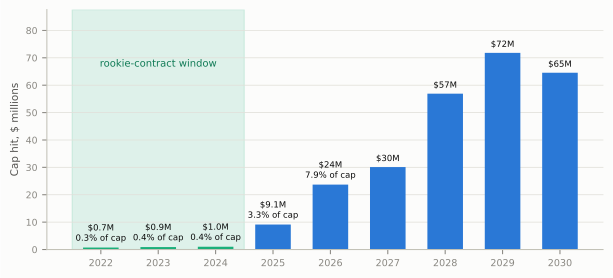
Figure 72.7: Brock Purdy’s cap hits, 2022–2030, in $ millions, with each year’s share of that year’s salary cap above the bar where the cap is known. The three rookie-contract seasons (shaded) cost the 49ers less than half a percent of the cap each. The five-year extension signed in May 2025 is shaped like most big contracts: a modest first year, then rising hits as the cap grows. Years after 2026 are as scheduled at signing and will change if the deal is restructured. Data: Over the Cap via nflverse.

What to notice: what the window bought. A top-ten quarterback contract costs about 22% of the cap (Figure 72.1); Purdy cost under half a percent, so the 49ers had a fifth of their cap to spend elsewhere. In 2023 they paid Christian McCaffrey, Nick Bosa, Trent Williams, Fred Warner, George Kittle and Deebo Samuel at the same time, and they reached the Super Bowl. (Whether Purdy or Kyle Shanahan’s system earned those numbers is the “system quarterback” debate of Quarterback Play; the cap didn’t care.) As a seventh-rounder Purdy had no fifth-year option, so the window was always going to close once he became eligible for an extension after his third season. In May 2025 it closed: a five-year extension worth up to $265 million, $53 million a year, about 19% of the cap when signed, with $100 million fully guaranteed at signing. The same team, in the same two drafts, paid three first-round picks for the quarterback the Johnson chart loved and got its starter with a pick no chart valued at all. The lesson is not that late picks beat early ones; it is how uncertain the draft is, and why surplus value says to collect more chances rather than pay heavily for one.

Evaluating players: what scouts grade, and what the stopwatch can’t see

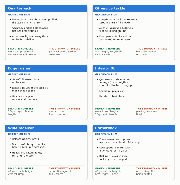
Every pick starts with an evaluation, and the core of evaluation is still film: area scouts watch every snap a prospect played in college and grade him against what his position demands. Figure 72.8 is a condensed version of the traits most NFL scouting departments grade.

CARDS = [
    ("Quarterback", ["Processing: reads the coverage, finds\nthe open man on time",
                     "Accuracy and ball placement,\nnot just completion %",
                     "Arm: velocity and every throw\nto the far sideline"],
     "hand size (grip in cold,\nwet weather); little else", "poise when the pocket\ncollapses"),
    ("Offensive tackle", ["Length: arms 34 in. or more to\nkeep rushers off his body",
                          "Anchor: absorbs a bull rush\nwithout giving ground",
                          "Feet: pass sets (kick-slide,\njump sets) to mirror speed"],
     "arm length, 10-yd split,\nshort shuttle", "hand timing and\nrecovery"),
    ("Edge rusher", ["Get-off: first-step burst\nat the snap",
                     "Bend: dips under the tackle's\nreach at full speed",
                     "Hands and a plan:\nmoves and counters"],
     "10-yard split, 3-cone,\nlength", "motor in the\nfourth quarter"),
    ("Interior DL", ["Quickness to shoot a gap\n(one-gap) or strength to\ncontrol a blocker (two-gap)",
                     "Leverage: plays low",
                     "Hands to shed blocks"],
     "weight, arm length,\n10-yd split, bench", "playing low when\ntired"),
    ("Wide receiver", ["Release against press",
                       "Route craft: tempo, breaks,\nhow he sets up a defender",
                       "Hands and catch radius;\nrun after the catch"],
     "40-yard dash, height,\nvertical jump", "separation against\nNFL corners"),
    ("Cornerback", ["Press, mirror and hip turn:\nopens to run without a false step",
                    "Long speed: can run with\na go route for 40 yards",
                    "Ball skills; eyes in zone;\ntackling in run support"],
     "40-yard dash, height,\narm length, 3-cone", "recovering after\nbeing beaten"),
]
fig, ax = plt.subplots(figsize=(6.6, 6.8))
ax.set_xlim(0, 2)
ax.set_ylim(0, 3)
ax.axis("off")
for i, (pos, traits, proxy, unseen) in enumerate(CARDS):
    col, row = i % 2, 2 - i // 2
    x0, y0 = col + 0.03, row + 0.04
    ax.add_patch(FancyBboxPatch((x0, y0), 0.94, 0.92, boxstyle="round,pad=0.0,rounding_size=0.03",
                                fc=style.SURFACE, ec=style.BASELINE, lw=0.9))
    ax.add_patch(Rectangle((x0, y0 + 0.8), 0.94, 0.12, fc=style.OFFENSE, ec="none"))
    ax.text(x0 + 0.03, y0 + 0.86, pos, fontsize=8.6, fontweight="bold", color="white", va="center")
    ax.text(x0 + 0.03, y0 + 0.75, "GRADED ON FILM", fontsize=5.8, color=style.OFFENSE_DARK, fontweight="bold")
    yy = y0 + 0.70
    for t in traits:
        nl = t.count("\n") + 1
        ax.text(x0 + 0.05, yy, "• " + t.replace("\n", "\n   "), fontsize=6.4, color=style.INK, va="top")
        yy -= 0.058 * nl + 0.025
    ax.plot([x0 + 0.03, x0 + 0.91], [y0 + 0.235, y0 + 0.235], color=style.GRID, lw=0.8)
    ax.text(x0 + 0.03, y0 + 0.205, "STAND-IN NUMBERS", fontsize=5.8, color=GREEN, fontweight="bold", va="top")
    ax.text(x0 + 0.03, y0 + 0.165, proxy, fontsize=6.2, color=style.INK_2, va="top")
    ax.text(x0 + 0.50, y0 + 0.205, "THE STOPWATCH MISSES", fontsize=5.8, color=style.DEFENSE_DARK,
            fontweight="bold", va="top")
    ax.text(x0 + 0.50, y0 + 0.165, unseen, fontsize=6.2, color=style.INK_2, va="top")
fig.tight_layout()
plt.show()

Figure 72.8: What scouts grade, position by position (a composite of common scouting criteria, not one team’s form). For each position: the traits that decide the grade, the measurement or drill that stands in for them, and what no stopwatch can see. Notice how much of each card is about processing, technique and movement in pads rather than raw speed: that is why the combine adjusts grades rather than sets them. The drills named under ‘stand-in numbers’ are explained in the next section.

A few words on those cards are terms of art. A lineman’s anchor is his ability to stop a bull rush, sinking his weight and holding his ground instead of being driven back into the quarterback (Pass Protection). An edge rusher’s get-off is his first-step explosion at the snap, and bend is his ability to dip his shoulder and turn the corner around a tackle at full speed without slowing down (The Pass Rush). Processing, for a quarterback, is how quickly he reads the coverage and knows where to throw. Motor is effort that doesn’t fade late in games; hand timing is when a tackle shoots his punch, too early and the rusher swats it away, too late and he is already beaten; catch radius is how far from his body a receiver can still catch the ball. Hand size is the quarterback’s only real stand-in number because scouts believe a bigger hand holds a cold, wet ball better and fumbles less. Notice that the first trait on almost every card is one no stopwatch measures.

The combine and pro days

Film is graded through the fall. In February and March come the measurements. The NFL Scouting Combine brings more than 300 invited prospects (319 in 2026) to Indianapolis, where it has been held since 1987, for a week of medical exams, interviews with teams, body measurements (height, weight, arm length, hand size) and timed drills.¹⁸ Each drill stands in for a football trait:

• 40-yard dash, with a 10-yard split: long speed for receivers, backs and corners; the split, the first ten yards, is the closest number to a lineman’s or edge rusher’s burst off the snap.
• Vertical and broad jump: lower-body explosiveness.
• Bench press (reps of 225 pounds): upper-body strength endurance, mostly for linemen.
• Three-cone drill and 20-yard short shuttle: change of direction, the ability to stop, bend and restart, which matters for edge rushers turning the corner and corners mirroring routes.

A pro day is the campus version, held in March and April for a school’s prospects with NFL scouts and coaches watching. Players who skipped drills at the combine run them here, usually on their own familiar turf and often with friendlier timing, so experienced evaluators treat pro-day numbers as slightly optimistic.

RAS: putting the numbers on one scale

A 4.6 forty is slow for a cornerback and astonishing for a 300-pound tackle, so raw numbers can’t be compared across positions. RAS, the Relative Athletic Score created by the analyst Kent Lee Platte, solves that by converting each measurement into a percentile among every player measured at the same position since 1987, then combining them into one score from 0 to 10. A 5 is average for the position; 8 is very good; 9 and above is elite.¹⁹

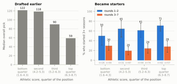
Is it useful? Figure 72.9 builds a simplified RAS-style score from the nflverse combine data and asks what it predicts.

COMB = nfl().load_combine().to_pandas()


def _inches(s):
    try:
        f_, i_ = str(s).split("-")
        return int(f_) * 12 + int(i_)
    except ValueError:
        return np.nan


COMB["htin"] = COMB.ht.map(_inches)
POSGRP = {"DE": "Edge", "EDGE": "Edge", "CB": "Cornerback"}
MEAS = {"htin": 1, "wt": 1, "forty": -1, "vertical": 1, "broad_jump": 1, "bench": 1, "cone": -1, "shuttle": -1}
cmb = COMB[COMB.pos.isin(POSGRP)].copy()
cmb["grp"] = cmb.pos.map(POSGRP)
for k, sgn in MEAS.items():
    cmb[k + "_p"] = cmb.groupby("grp")[k].transform(lambda s, sgn=sgn: (sgn * s).rank(pct=True))
cmb["nmeas"] = cmb[list(MEAS)].notna().sum(axis=1)
cmb["score"] = 10 * cmb[[k + "_p" for k in MEAS]].mean(axis=1)
cmb = cmb[(cmb.nmeas >= 5) & cmb.season.between(2006, 2018) & cmb.pfr_id.notna()]
dp = DRAFT_PICKS.dropna(subset=["pfr_player_id"]).drop_duplicates("pfr_player_id")
RAS = cmb.merge(dp[["pfr_player_id", "pick", "round", "seasons_started"]], left_on="pfr_id",
                right_on="pfr_player_id", how="inner")
BANDS = ["bottom\nquarter", "second", "third", "top\nquarter"]
RAS["band"] = RAS.groupby("grp").score.transform(lambda s: pd.qcut(s, 4, labels=False))
RAS["band"] = pd.Categorical.from_codes(RAS.band.astype(int), BANDS)
RAS["early"] = np.where(RAS["round"] <= 2, "rounds 1–2", "rounds 3–7")
RAS["starter3"] = RAS.seasons_started.fillna(0) >= 3
R_RAS_PICK = np.corrcoef(RAS.score, RAS.pick)[0, 1]
# What score range each quarter covers (pooled; the quarters are cut within each position, so this is a guide)
_cuts = RAS.groupby("band", observed=True).score.agg(["min", "max"])
BAND_TICKS = [f"{b}\n({lo:.1f}–{hi:.1f})" for b, (lo, hi) in zip(BANDS, _cuts.values)]

fig, (a1, a2) = plt.subplots(1, 2, figsize=(6.6, 3.2), gridspec_kw=dict(width_ratios=[1, 1.25]))
mp = RAS.groupby("band", observed=True).pick.median()
a1.bar(range(len(mp)), mp.values, color=style.MUTED, width=0.6, zorder=2)
for i, v in enumerate(mp.values):
    a1.text(i, v + 3, f"{v:.0f}", ha="center", fontsize=7, color=style.INK)
a1.set_xticks(range(len(mp)))
a1.set_xticklabels(BAND_TICKS, fontsize=6.4)
a1.set_xlabel("Athletic score, quarter of the position", fontsize=7.5)
a1.set_ylabel("Median overall pick", fontsize=7.5)
a1.set_title("Drafted earlier", fontsize=8.5)
a1.grid(axis="x", visible=False)
tab = RAS.groupby(["early", "band"], observed=True).agg(rate=("starter3", "mean"), n=("starter3", "size")).reset_index()
for j, (grp, c) in enumerate((("rounds 1–2", style.OFFENSE), ("rounds 3–7", style.SERIES[1]))):
    t = tab[tab.early == grp]
    xs = np.arange(len(t)) + (j - 0.5) * 0.36
    se = 100 * 1.96 * np.sqrt(t.rate * (1 - t.rate) / t.n)       # 95% interval for each share
    a2.bar(xs, 100 * t.rate, 0.34, color=c, label=grp, zorder=2)
    a2.errorbar(xs, 100 * t.rate, yerr=se, fmt="none", ecolor=style.INK_2, elinewidth=0.8, capsize=2, zorder=3)
    for xv, (r_, n_, e_) in zip(xs, zip(t.rate, t.n, se)):
        a2.text(xv, 100 * r_ + e_ + 1.5, f"{100 * r_:.0f}", ha="center", fontsize=6.4, color=style.INK)
        a2.text(xv, -6.5, f"n={n_}", ha="center", fontsize=5.4, color=style.MUTED)
a2.set_xticks(range(4))
a2.set_xticklabels(BAND_TICKS, fontsize=6.4)
a2.set_ylim(-9, 108)
a2.set_ylabel("% who started 3+ seasons", fontsize=7.5)
a2.set_xlabel("Athletic score, quarter of the position", fontsize=7.5)
a2.set_title("Became starters", fontsize=8.5)
a2.legend(fontsize=6.8, loc="upper left")
a2.grid(axis="x", visible=False)
for ax in (a1, a2):
    ax.tick_params(labelsize=7)
fig.tight_layout()
plt.show()
_e = tab[tab.early == "rounds 1–2"].set_index("band")
RAS_LO, RAS_HI = _e.rate.iloc[0], _e.rate.iloc[-1]
RAS_N_LO, RAS_N_HI = int(_e.n.iloc[0]), int(_e.n.iloc[-1])
RAS_CI = 100 * 1.96 * np.sqrt(RAS_LO * (1 - RAS_LO) / RAS_N_LO)      # +/- points on the smaller bar

Figure 72.9: What an athletic score predicts, and what it doesn’t. A simplified RAS-style score (each of height, weight, 40-yard dash, vertical, broad jump, bench, three-cone and shuttle converted to a percentile within the position, averaged and scaled 0–10; at least five measurements required) for edge rushers and cornerbacks at the 2006–2018 combines who were drafted. Left: better athletes are drafted earlier: teams already price athleticism in. Both panels split the players into quarters by their score within the position. Tick labels give each quarter’s range of scores. Right: the share who became starters for three or more seasons, split by when they were drafted, with 95% intervals (the thin bars). Within each draft-round group the top quarter did start more often than the bottom quarter, but each bar is only a few dozen players and the intervals overlap widely: the score adds something after the draft order is set, but far less precisely than the bars alone suggest. Data: nflverse combine and draft-pick data (Pro Football Reference).

The left panel shows that teams already draft by athleticism: the correlation between the score and the pick number is -0.34 (negative because a better score means an earlier, lower-numbered pick). The right panel is more interesting than a shrug. Among players taken in the first two rounds, the top quarter of athletes became three-year starters 71% of the time and the bottom quarter 50%, which looks like a big edge. But those bars are 62 and 26 players, so each is uncertain by about 19 percentage points either way, and the gap could be much smaller than it looks. A fair reading: athleticism still helps a little after teams have priced it in, and nobody should bet heavily on the size of that help. Athletic scores tell you who can play the position at NFL speed; they can’t tell you who processes a coverage, plays with his hands, or keeps improving. So treat RAS as a filter, not a ranking: a very low score at a premium position is a real warning, and a very high score on a player with thin film is a bet on coaching. Some players beat their numbers for a career. Others, the “workout warriors,” turn a great combine into a high pick and never play like it.

Scheme fit: the same player, different value

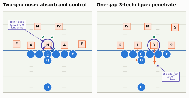
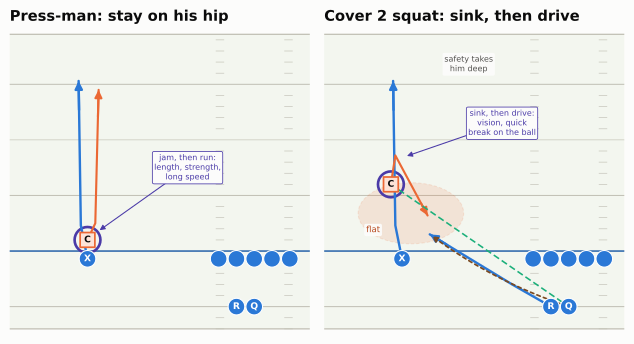
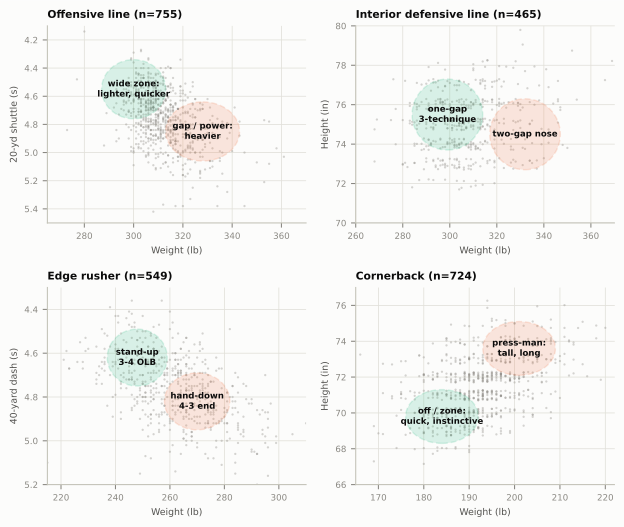
Here is where X’s and O’s come back. Scheme fit is how well a player’s body and skills match what a particular scheme asks of his position. Because schemes ask different things, the same prospect can be a first-round talent on one board and a fourth-rounder on another, and a smart team shops where its scheme makes it the only serious buyer.

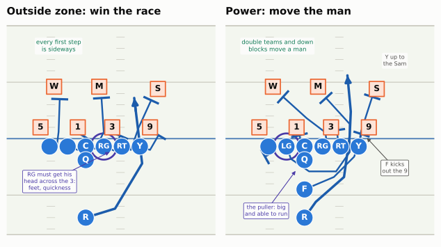
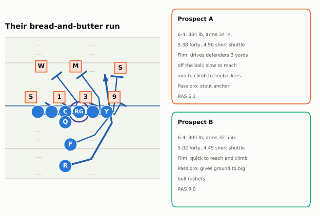
Offensive line: move your feet or move the man

def O(key, pos, d, w, label=None):
    return Player(key, pos, "off", d, w, label=key if label is None else label)


def D(key, pos, d, w, label=None):
    return Player(key, pos, "def", d, w, label=label)


def oline(show=("C",)):
    """Five offensive linemen; only the ones in `show` carry a label."""
    return [O(k, k, -0.7, w, k if k in show else "")
            for k, w in zip(["LT", "LG", "C", "RG", "RT"], (-3.2, -1.6, 0.0, 1.6, 3.2))]


def clean(ax):
    """Zoomed diagrams: drop the yard numbers (they would sit outside the window) and clip all text."""
    for t in list(ax.texts):
        if t.get_text().isdigit() and t.get_alpha() == 0.55:
            t.remove()
        else:
            t.set_clip_on(True)


def fdraw(p, ax, **kw):
    fld = p.draw(ax=ax, **kw)
    clean(ax)
    return fld


def go_to(p, key, end, kind="block", via=(), speed=None, delay=0.0):
    """Move `key` through absolute (d, w) points `via` to `end`, as a block, path or run."""
    start = np.array(p._cur(key))
    pts = [tuple(np.array(q) - start) for q in (*via, end)]
    if kind == "block":
        return p.block(key, pts=pts, speed=speed, delay=delay)
    return {"path": p.path, "run": p.run, "pull": p.pull}[kind](key, pts, speed=speed, delay=delay)


def fsay(fld, p, d, w, text, color=style.INK_2, fontsize=7.0, ha="center", bold=False):
    x, y = fld.xy(*p.to_abs(d, w))
    fld.ax.text(x, y, text, fontsize=fontsize, color=color, ha=ha, va="center", zorder=9,
                fontweight="bold" if bold else "normal",
                bbox=dict(boxstyle="round,pad=0.22", fc=style.SURFACE, ec="none", alpha=0.93))


def fpoint(fld, p, frm, to, text, color=style.INK_2, fontsize=6.8, ha="center"):
    (x0, y0), (x1, y1) = fld.xy(*p.to_abs(*frm)), fld.xy(*p.to_abs(*to))
    fld.ax.annotate("", (x1, y1), (x0, y0), zorder=8,
                    arrowprops=dict(arrowstyle="-|>", color=color, lw=0.8, shrinkA=6, shrinkB=4, mutation_scale=8))
    fld.ax.text(x0, y0, text, fontsize=fontsize, color=color, ha=ha, va="center", zorder=9,
                bbox=dict(boxstyle="round,pad=0.22", fc=style.SURFACE, ec=color, lw=0.6))


def pair(width=6.6, height=4.6):
    fig, axes = plt.subplots(1, 2, figsize=(width, height))
    return fig, axes

A wide-zone team and a gap team ask their linemen to do opposite things. Outside zone (wide zone) asks every lineman to step sideways at the snap and reach the defender in front of him: to get his body across a man who is already lined up outside him. That is a race, and it rewards quick feet, balance and athleticism over size. A gap scheme such as power asks the play-side linemen to down block, driving a defender sideways off his spot from an angle, and asks a guard to pull and lead through the hole. That rewards mass and power, plus one guard who can run. Figure 72.10 puts the two side by side.

def front_43():
    return [D("LE", "DE", 1.0, technique("5", -1), "5"), D("LT1", "DT", 1.0, technique("1", -1), "1"),
            D("R3", "DT", 1.0, technique("3", 1), "3"), D("RE", "DE", 1.0, technique("9", 1), "9"),
            D("WILL", "WILL", 4.6, -2.8, "W"), D("MIKE", "MIKE", 4.6, 1.2, "M"), D("SAM", "SAM", 4.4, 6.4, "S")]


def ol_base(fb=False, show=("C",)):
    off = oline(show) + [O("Y", "TE", -0.7, 4.8, "Y"), O("QB", "QB", -1.9, 0.0, "Q"), O("RB", "RB", -7.0, 0.0, "R")]
    if fb:
        off += [O("FB", "FB", -4.5, 0.0, "F")]
    return off


LAT, WIN = (-6.5, 11.0), (-8.5, 10.0)
fig, (axl, axr) = pair(6.7, 5.0)
p = Play(ol_base(show=("C", "RG", "RT")), front_43(), los=35, to_go=None, title="Outside zone: win the race")
# wide-zone rules against this front: C + RG combo the 3 (RG keeps him, C climbs to the Mike), the uncovered RT
# climbs to the Sam, Y reaches the 9, LG cuts off the 1, LT climbs to the Will; the backside 5 is left alone.
go_to(p, "LT", (3.5, -2.3), via=[(-1.0, -2.6), (0.6, -2.4)])
go_to(p, "LG", (0.1, 0.0), via=[(-1.0, -0.7)])
go_to(p, "C", (3.6, 1.4), via=[(-0.9, 0.9), (0.6, 1.6)])
go_to(p, "RG", (0.25, 3.05), via=[(-1.05, 2.5)])
go_to(p, "RT", (3.4, 5.8), via=[(-1.0, 4.0), (1.0, 4.7)])
go_to(p, "Y", (0.3, 6.45), via=[(-1.0, 5.7)])
go_to(p, "RB", (3.6, 4.3), "run", via=[(-6.2, 2.6), (-2.2, 5.0)])
p.handoff("RB", t=0.6)
p.highlight("RG", color=PURPLE)
f = fdraw(p, axl, lateral=LAT, window=WIN)
fsay(f, p, 8.2, -2.4, "every first step\nis sideways", fontsize=6.4, color=GREEN)
fpoint(f, p, (-3.8, -3.2), (-1.05, 2.4), "RG must get his\nhead across the 3:\nfeet, quickness", color=PURPLE,
       fontsize=6.0)

# power right against the same front: RG + RT double the 3 and RG comes off to the Will, C blocks back on the 1,
# the fullback kicks out the end man on the line (the 9), Y climbs to the Sam, and the left guard pulls up
# through the hole for the Mike
p2 = Play(ol_base(fb=True, show=("C", "LG", "RG", "RT")), front_43(), los=35, to_go=None,
          title="Power: move the man")
go_to(p2, "RT", (0.75, 2.85), via=[(-0.3, 3.0)])
go_to(p2, "RG", (3.7, -1.9), via=[(-0.25, 1.95), (0.55, 1.85), (1.8, 0.2)])
go_to(p2, "C", (0.3, -0.45), via=[(-0.5, -0.25)])
go_to(p2, "LT", (-1.6, -3.5), via=[(-1.1, -2.6)])
go_to(p2, "Y", (3.7, 6.0), via=[(0.6, 5.0)])
go_to(p2, "FB", (0.4, 5.05), via=[(-3.4, 2.6), (-1.6, 4.4)])
go_to(p2, "LG", (3.6, 1.9), "pull", via=[(-1.8, -1.2), (-2.9, 0.4), (-2.9, 2.8), (-1.2, 4.0), (1.3, 4.0)])
go_to(p2, "RB", (5.6, 3.8), "run", via=[(-5.6, 1.0), (-3.4, 3.5), (0.2, 4.0), (2.4, 4.1)])
p2.handoff("RB", t=0.9)
p2.highlight("LG", color=PURPLE)
f2 = fdraw(p2, axr, lateral=LAT, window=WIN)
fsay(f2, p2, 8.2, -2.4, "double teams and down\nblocks move a man", fontsize=6.4, color=GREEN)
fpoint(f2, p2, (-6.4, -3.4), (-2.6, -0.6), "the puller: big\nand able to run", color=PURPLE, fontsize=6.0)
fpoint(f2, p2, (-2.6, 8.0), (0.3, 5.3), "F kicks\nout the 9", fontsize=6.0)
fsay(f2, p2, 6.9, 8.0, "Y up to\nthe Sam", fontsize=6.0)
fig.tight_layout()
plt.show()

Figure 72.10: Why a wide-zone team and a gap team draft different linemen (illustrative, against the same 4-3 front with the strength to the tight end). Left, outside zone right: every blocker’s first step is sideways. The right guard (ringed) has to get his body across a 3-technique who starts outside him while the center steps with him and then climbs to the Mike; the uncovered right tackle climbs to the Sam, the tight end reaches the 9, and the backside end (5) is left alone, because the back is running away from him. That is a race won with feet and quickness. Right, power right: the right guard and tackle double-team the 3-technique and drive him off the ball, then the guard comes off to the Will; the center blocks back on the 1, the fullback kicks out the end man on the line (the 9), the tight end climbs to the Sam, and the left guard (ringed) pulls around and leads through the hole for the Mike. Those blocks are won with mass and leg drive, and the puller is a big man who must also run. Typical builds: wide-zone linemen often weigh about 295–315 pounds, gap linemen 315–340.

That’s why a wide-zone team will happily draft a 300-pound guard who ran well in the shuttle and a gap team will pass on him for a 330-pounder who moves people. The weights in the caption are rough tendencies, not rules: teams draft for what the player does on film, and a heavy man who moves well fits anywhere. (The 49ers film room below shows how small the real difference in average weight is.)

Defensive line: two-gap nose or one-gap 3-technique

The same split runs through the defensive front. In a two-gap defense, often a 3-4 with a nose tackle head-up on the center, the lineman’s job is to strike the blocker, control him, and be ready to shed into either gap beside him (two-gap play). In a one-gap attacking front, the 3-technique on the guard’s outside shoulder owns a single gap and shoots into it at the snap (one-gap play). DL Techniques and Gap Control taught both jobs; Figure 72.11 shows what each asks of a body.

def threefour():
    return [D("LE", "DE", 1.0, technique("4", -1), "4"), D("NT", "NT", 1.0, 0.0, "N"),
            D("RE", "DE", 1.0, technique("4", 1), "4"),
            D("LOLB", "OLB", 1.2, -5.9, "E"), D("ROLB", "OLB", 1.2, 6.5, "E"),
            D("LILB", "ILB", 4.6, -1.9, "M"), D("RILB", "ILB", 4.6, 2.1, "W")]


def fourman():
    return front_43()


fig, (axl, axr) = pair(6.7, 4.2)
off = oline() + [O("Y", "TE", -0.7, 4.8, "Y"), O("QB", "QB", -1.9, 0.0, "Q"), O("RB", "RB", -7.0, 0.0, "R")]
p = Play(off, threefour(), los=35, to_go=None, title="Two-gap nose: absorb and control")
go_to(p, "C", (0.0, 0.0)); go_to(p, "RG", (-0.05, 0.85), via=[(-0.5, 1.3)])
p.highlight("NT", color=PURPLE)
f = fdraw(p, axl, lateral=(-8.0, 8.0), window=(-8.0, 7.5))
for w in (-1.0, 1.0):     # the nose owns both A gaps: he can shed to either side
    (x0, y0), (x1, y1) = f.xy(*p.to_abs(0.95, 0.35 * np.sign(w))), f.xy(*p.to_abs(0.15, w))
    f.ax.add_patch(FancyArrowPatch((x0, y0), (x1, y1), arrowstyle="-|>", mutation_scale=9, color=PURPLE, lw=1.6,
                                   zorder=8))
    fsay(f, p, 2.55, 0.85 * np.sign(w), "A", color=GREEN, fontsize=6.6, bold=True)
fpoint(f, p, (4.9, -5.8), (1.5, -0.5), "both A gaps:\nmass, anchor,\nlong arms", color=PURPLE, fontsize=6.0)

p2 = Play(off, fourman(), los=35, to_go=None, title="One-gap 3-technique: penetrate")
go_to(p2, "R3", (-2.6, 2.5), "path", via=[(0.2, 2.45)], speed=4.0)
go_to(p2, "LT1", (-2.2, -0.85), "path", via=[(0.2, -0.8)], speed=4.0)
p2.highlight("R3", color=PURPLE)
f2 = fdraw(p2, axr, lateral=(-8.0, 8.0), window=(-8.0, 7.5))
fsay(f2, p2, 2.55, 2.4, "B", color=GREEN, fontsize=6.6, bold=True)
fpoint(f2, p2, (-5.0, 5.6), (-2.5, 2.7), "one gap, fast:\nget-off,\nquickness", color=PURPLE, fontsize=6.0)
fig.tight_layout()
plt.show()

Figure 72.11: Two defensive-line jobs, two body types (illustrative). Left, a two-gap 3-4 (E: the stand-up edge players, its outside linebackers): the nose (ringed) lines up head-up on the center and must absorb him, often a guard as well, and still be able to shed into either A gap. He needs mass, a strong anchor and long arms, so classic two-gap noses are often 320–340 pounds or more. Right, a one-gap four-man front: the 3-technique (ringed) is shaded on the right guard’s outside shoulder and attacks the B gap at the snap. He needs first-step quickness and leverage more than bulk, so he is often 285–315 pounds. A team switching from one front to the other has to rebuild its defensive line.

Pure two-gap 3-4 defenses are rare now, but the heavy nose came back another way: the tite front (Odd and Hybrid Fronts) puts a nose on the center and two linemen on the tackles’ inside shoulders to wall off inside runs, and it needs a big man in the middle again. The Eagles drafted both archetypes in back-to-back first rounds: Jordan Davis (No. 13 in 2022, 341 pounds at the combine), a nose, and Jalen Carter (No. 9 in 2023, 314 pounds), a penetrating 3-technique.²⁰

The edge has the same split. A 4-3 defensive end plays with his hand in the dirt and must hold up against tackles in the run game, so teams like him heavier, around 255–280 pounds; a 3-4 outside linebacker stands up, rushes from wider and sometimes drops into coverage, so he can be lighter and quicker, around 240–260. But defenses played their base personnel on only about 30 percent of snaps in 2025, and spent the rest with five or more defensive backs,²¹ so whatever the base front is called, the live split today is less “4-3 end or 3-4 linebacker” than “run-down edge or pass-rush specialist”.

Cornerbacks: press or off

Cornerbacks split by technique, not by man versus zone. A team whose corners play press, jamming the receiver at the line, wants long, physical corners with the hips to turn and the long speed to run with a go route, whether they then play man or bail into a zone. Pete Carroll’s Seattle teams of the 2010s, the league’s signature press Cover 3 defense (Coverage Fundamentals), drafted outside corners with long arms and nearly all of them six feet or taller.²² A team whose corners play off coverage, with a cushion and their eyes in the backfield, can live with shorter corners who read the play and break on the ball quickly. The clearest case is the Cover 2 squat corner, who sits about five to seven yards off, keeps the flat and hands the deep ball to a safety: Ronde Barber, listed at 5 feet 10, played that role in Tampa Bay’s Tampa 2 on his way to the Hall of Fame.²³ Figure 72.12 shows both jobs.

def cb_play(press=True):
    off = oline(()) + [O("QB", "QB", -5.0, 0.0, "Q"), O("X", "WR", -0.7, -15.0, "X"),
                       O("RB", "RB", -5.0, -1.6, "R")]
    dfn = [D("CB", "CB", 1.0 if press else 6.0, -15.0 if press else -16.0, "C")]
    p = Play(off, dfn, los=35, to_go=None,
             title="Press-man: stay on his hip" if press else "Cover 2 squat: sink, then drive")
    p.route("X", [(3, 0.6), (16, 0.8)], side=None)
    if press:
        go_to(p, "CB", (14.5, -14.0), "path", via=[(2.5, -14.3)], speed=7.0)
    else:
        p.route("RB", [(2.0, -3.5), (6.5, -10.9)], frame="field")
        go_to(p, "CB", (3.2, -12.7), "path", via=[(8.6, -15.6)], speed=4.2)
        p.zone((3.4, -14.2), (5.5, 9.5))
        p.read("QB", key="CB")
        p.pass_to("RB", t=1.6)
    p.highlight("CB", color=PURPLE)
    return p


LAT_CB, WIN_CB = (-21.5, 4.5), (-7.0, 19.5)
fig, (axl, axr) = pair(6.7, 4.6)
p = cb_play(True)
f = fdraw(p, axl, lateral=LAT_CB, window=WIN_CB)
fpoint(f, p, (7.5, -6.0), (1.6, -14.3), "jam, then run:\nlength, strength,\nlong speed", color=PURPLE, fontsize=6.0)
p2 = cb_play(False)
f2 = fdraw(p2, axr, lateral=LAT_CB, window=WIN_CB)
fpoint(f2, p2, (11.5, -6.0), (8.4, -15.0), "sink, then drive:\nvision, quick\nbreak on the ball", color=PURPLE,
       fontsize=6.0)
fsay(f2, p2, 16.8, -9.0, "safety takes\nhim deep", fontsize=6.0)
fsay(f2, p2, 1.9, -17.6, "flat", fontsize=6.4, color=style.DEFENSE_DARK)
fig.tight_layout()
plt.show()

Figure 72.12: Two cornerback jobs (illustrative; the outside receiver on the offense’s left). Left, press-man: the corner (ringed) is a yard off the receiver, jams him, then turns and runs with him on his hip, no matter where he goes. Length, strength and long speed decide it. Right, a Cover 2 squat corner: he lines up six yards off with outside leverage, reroutes the receiver, sinks a few yards while the safety takes the go route over the top, and drives on the throw to the running back in the flat. The dashed line is his eyes, on the quarterback. Vision, footwork and a quick break on the ball decide it, so a shorter corner can thrive.

The archetypes, in real numbers

Figure 72.13 puts real combine measurements behind these archetypes. Each dot is one prospect; the shaded regions are drawn by hand to show where each kind of team tends to shop. They are a picture of the idea, not a finding: the 49ers film room below checks the offensive-line version against what teams actually drafted.

c = COMB[COMB.season.between(2006, 2026)].copy()
# combine "OLB" mixes 3-4 rushers with off-ball 4-3 linebackers: keep only OLBs who became NFL pass rushers
_sacks = DRAFT_PICKS.dropna(subset=["pfr_player_id"]).drop_duplicates("pfr_player_id").set_index("pfr_player_id").def_sacks
c["nfl_sacks"] = c.pfr_id.map(_sacks).fillna(0)
edge = c[c.pos.isin(["DE", "EDGE"]) | ((c.pos == "OLB") & (c.nfl_sacks >= 10))]
panels = [
    ("Offensive line", c[c.pos.isin(["OT", "OG", "C", "OL", "G"])], "wt", "shuttle", "Weight (lb)", "20-yd shuttle (s)",
     [((300, 4.55), 26, 0.42, "wide zone:\nlighter, quicker", style.THIRD),
      ((328, 4.85), 30, 0.42, "gap / power:\nheavier", style.SERIES[1])], (265, 370), (4.1, 5.5)),
    ("Interior defensive line", c[c.pos.isin(["DT", "NT"])], "wt", "htin", "Weight (lb)", "Height (in)",
     [((332, 74.5), 30, 3.6, "two-gap nose", style.SERIES[1]),
      ((299, 75.5), 30, 3.6, "one-gap\n3-technique", style.THIRD)], (260, 370), (70, 80)),
    ("Edge rusher", edge, "wt", "forty", "Weight (lb)", "40-yard dash (s)",
     [((270, 4.82), 24, 0.26, "hand-down\n4-3 end", style.SERIES[1]),
      ((248, 4.62), 22, 0.26, "stand-up\n3-4 OLB", style.THIRD)], (215, 310), (4.3, 5.2)),
    ("Cornerback", c[c.pos.isin(["CB"])], "wt", "htin", "Weight (lb)", "Height (in)",
     [((201, 73.6), 16, 3.0, "press-man:\ntall, long", style.SERIES[1]),
      ((184, 69.8), 16, 3.0, "off / zone:\nquick, instinctive", style.THIRD)], (165, 222), (66, 77)),
]
fig, axes = plt.subplots(2, 2, figsize=(6.6, 5.6))
for ax, (title, d_, xc, yc, xl, yl, regions, xlim, ylim) in zip(axes.flat, panels):
    d_ = d_.dropna(subset=[xc, yc])
    jit = np.random.default_rng(0).uniform(-0.3, 0.3, len(d_)) if yc == "htin" else 0
    ax.scatter(d_[xc], d_[yc] + jit, s=3, color=style.MUTED, alpha=0.35, lw=0, zorder=2)
    for (cx, cy), w_, h_, lab, col in regions:
        ax.add_patch(Ellipse((cx, cy), w_, h_, fc=col, alpha=0.16, ec=col, lw=1.1, ls=(0, (4, 2)), zorder=3))
        ax.text(cx, cy, lab, ha="center", va="center", fontsize=6.4, color=style.INK, zorder=4, fontweight="bold")
    ax.set_title(f"{title} (n={len(d_)})", fontsize=8)
    ax.set_xlabel(xl, fontsize=7)
    ax.set_ylabel(yl, fontsize=7)
    ax.set_xlim(*xlim)
    ax.set_ylim(*ylim)
    ax.tick_params(labelsize=6.5)
    if yc in ("shuttle", "forty"):
        ax.invert_yaxis()
fig.tight_layout()
plt.show()

# A team-level check on the OL archetype: linemen drafted 2017-2025 by Shanahan-tree play-callers (49ers,
# Rams, Packers from 2019, Dolphins from 2022; PFR team codes) against everyone else's.
_ol = DRAFT_PICKS[DRAFT_PICKS.position.isin(["T", "G", "C", "OL", "OT", "OG"]) & DRAFT_PICKS.season.between(2017, 2025)]
_ol = _ol.merge(COMB[["pfr_id", "wt", "shuttle"]], left_on="pfr_player_id", right_on="pfr_id", how="left")
_ol["wz"] = (_ol.team.isin(["SFO", "LAR", "RAM"]) | ((_ol.team == "GNB") & (_ol.season >= 2019))
             | ((_ol.team == "MIA") & (_ol.season >= 2022)))
WZ = _ol.groupby("wz").agg(n=("pick", "size"), wt=("wt", "mean"), sh=("shuttle", "mean"))
SF_OL_WT = _ol[_ol.team == "SFO"].wt.mean()

Figure 72.13: Body types by position and scheme: every combine prospect measured 2006–2026 at four positions (dots), with the typical scheme archetypes shaded (illustrative regions, not hard cut-offs). Offensive linemen: wide-zone teams shop on the lighter, quicker side (upper left: the shuttle axis is flipped so faster times sit higher), gap teams on the heavier side. Interior defensive linemen (combine DT and NT; the generic ‘DL’ label used since 2018 is left out because it mixes ends and tackles): two-gap noses are the heaviest men in the draft; one-gap 3-techniques are 20 to 50 pounds lighter. Edge rushers (combine DE and EDGE, plus combine OLBs who went on to at least 10 NFL sacks, so that off-ball linebackers are left out): hand-down 4-3 ends are heavier than stand-up 3-4 outside linebackers. Cornerbacks: press-man teams want height (and length, which the combine measures but this data set does not include); off-coverage teams can take shorter players. Data: nflverse combine data (Pro Football Reference).

NoteFilm room: San Francisco 49ers, 2017–2025

The pattern: Kyle Shanahan’s 49ers run the purest wide-zone offense in the league (the Shanahan case study tells its history), and they have mostly filled their offensive line from the middle of the draft. From 2017 to 2025 they drafted ten offensive linemen; only two went in the first two rounds (Mike McGlinchey ninth overall in 2018 and Aaron Banks in the second round in 2021), and the rest came from rounds 3 to 7: Dominick Puni (third round, 2024), who started as a rookie, Spencer Burford (fourth, 2022), Colton McKivitz (fifth, 2020) and others.²⁴

What to notice: it isn’t that the 49ers draft small linemen. Their picks with combine weights average about 311 pounds. Widen the lens to all four Shanahan-tree offenses (the 49ers, the Rams, the Packers from 2019 and the Dolphins from 2022) and the archetype shows up, but faintly: their 40 drafted linemen averaged 311 pounds and a 4.67-second shuttle, against 314 pounds and 4.73 for everyone else. A few pounds and a few hundredths of a second: the real difference is movement on film (the ability to reach and climb), which a stopwatch barely catches. They buy it at mid-round prices and trust their coaching to turn those players into starters. And where positional value says to pay, they paid: in 2020 they traded for left tackle Trent Williams rather than wait for one to develop. Cheap, scheme-specific depth inside; a premium price at the premium position. That is positional value and scheme fit working together.

NoteFilm room: Philadelphia Eagles, 2014–2025

The Eagles took the opposite route to an elite line: they paid for it. Using the same contract data as Figure 72.2, Philadelphia’s offensive line took a larger share of its player spending than the league average in every season from 2014 to 2025, as Figure 72.14 shows. They spent picks on it too: Lane Johnson went fourth overall in 2013, and Landon Dickerson and Cam Jurgens in the second round in 2021 and 2022. But the line’s best bargains were developed: Jason Kelce was a sixth-round pick, and Jordan Mailata, an Australian rugby league player who had never played American football, a seventh-rounder in 2018, both under offensive line coach Jeff Stoutland, who held the job from 2013 through the 2025 season. The high spending is largely the price of keeping what they built: Kelce, Johnson, Mailata and Dickerson all signed second contracts in Philadelphia.²⁵ The Eagles case study tells how that line made the scheme possible.

phi = TEAMS.xs("PHI", level="abbr")["OL"]
lg = TEAMS.groupby(level="year")["OL"].mean()
fig, ax = plt.subplots(figsize=(6.4, 2.6))
ax.plot(lg.index, 100 * lg.values, color=style.MUTED, lw=2, marker="o", ms=3, label="league average")
ax.plot(phi.index, 100 * phi.values, color=style.OFFENSE, lw=2.4, marker="o", ms=3.5, label="Eagles")
ax.fill_between(phi.index, 100 * lg.values, 100 * phi.values, color=style.OFFENSE, alpha=0.1)
ax.set_ylabel("OL share of player\ncap spending (%)", fontsize=7.5)
ax.set_xticks(range(2014, 2026))
ax.tick_params(labelsize=7)
ax.set_ylim(10, 34)
ax.legend(fontsize=7, loc="upper left", ncol=2)
fig.tight_layout()
plt.show()

Figure 72.14: The Eagles’ offensive line as a share of the team’s player cap spending (blue) against the league average (grey), 2014–2025. Philadelphia was above the league in every season, and in half of them by five percentage points or more, roughly an extra starter’s salary committed to the line each year. Dead money is excluded. Data: Over the Cap contract histories via nflverse.

The 53, the 48 and the practice squad

The last layer of roster building is the rulebook for who may play on Sunday. A team carries up to 90 players in the spring and summer, cuts to 53 in late August, and then manages several lists at once. Figure 72.15 lays them out.

fig, ax = plt.subplots(figsize=(6.6, 4.3))
ax.set_xlim(0, 10)
ax.set_ylim(0, 7.0)
ax.axis("off")


def box(x, y, w, h, title, body, fc, ec, tc=style.INK, tsize=8.2):
    ax.add_patch(FancyBboxPatch((x, y), w, h, boxstyle="round,pad=0.02,rounding_size=0.12", fc=fc, ec=ec, lw=1.2))
    ax.text(x + 0.15, y + h - 0.2, title, fontsize=tsize, fontweight="bold", color=tc, va="top")
    ax.text(x + 0.15, y + h - 0.62, body, fontsize=6.6, color=style.INK_2, va="top", linespacing=1.35)


box(0.2, 0.25, 6.0, 6.35, "53-man roster", "", style.SURFACE, style.OFFENSE)
box(0.45, 2.1, 3.3, 3.2, "Game-day actives: 48",
    "dress and may play\n(at least 8 offensive linemen;\notherwise 47)", style.OFFENSE_TINT, style.OFFENSE)
box(3.95, 3.45, 2.05, 1.85, "Inactives", "the rest of the 53;\nannounced 90 min\nbefore kickoff",
    "#efeeea", style.BASELINE)
box(3.95, 2.1, 2.05, 1.15, "Emergency 3rd QB", "dresses; not one\nof the 48", "#e3f4ec", GREEN, GREEN, tsize=7.4)
box(0.45, 0.45, 5.55, 1.4, "Signed through the season", "every player on the 53 is under contract and paid weekly;\n"
    "cutting him exposes him to waivers (fewer than 4 accrued seasons)", "#f6f6f3", style.BASELINE)
box(6.6, 3.45, 3.2, 2.55, "Practice squad: 16 (+1)",
    "practices with the team, not on the 53;\nany team may sign one to its 53;\n+1 international player exemption",
    "#fdf3e6", GOLD)
box(6.6, 0.25, 3.2, 2.85, "Injured reserve (IR)",
    "off the 53, spot freed;\nmust miss 4+ games;\nup to 8 may return a season;\nthe rest are out for the year",
    "#fbe7e7", RED)
ax.annotate("", (2.4, 5.36), (6.6, 5.8), arrowprops=dict(arrowstyle="-|>", color=GOLD, lw=1.6,
                                                        connectionstyle="arc3,rad=-0.18"))
ax.text(8.2, 6.45, "elevation: 2 a game,\n3 times per player", ha="center", fontsize=6.4, color=style.INK,
        bbox=dict(boxstyle="round,pad=0.2", fc=style.SURFACE, ec=GOLD, lw=0.6))
ax.annotate("", (6.6, 1.7), (6.05, 1.2), arrowprops=dict(arrowstyle="-|>", color=RED, lw=1.4))
fig.tight_layout()
plt.show()

Figure 72.15: How an NFL roster is organized during the season (rules as of 2026). The 53-man roster is the pool; on game day up to 48 of them may be active (if at least eight are offensive linemen), with the rest inactive. A third quarterback from the 53 may also dress as the emergency third quarterback without counting toward the 48. The practice squad (16 players, plus an international player exemption) practices with the team and can be elevated for a game, two a game and up to three times per player per season. Injured reserve removes a player from the 53 (red arrow); he must miss at least four games, and a team may bring back up to eight players a season. The gold arrow is an elevation from the practice squad to the game-day roster.

Game-day actives. A team may dress 48 of its 53, provided at least eight are offensive linemen (otherwise 47); the rest are declared inactive about 90 minutes before kickoff. Who sits is a weekly game-plan decision. A team facing a run-heavy opponent might dress a fifth defensive tackle instead of a sixth receiver, and the inactive list on Sunday morning is one of the best free clues to the plan.

The practice squad. Each team keeps 16 players on its practice squad (plus one exemption for an international player). They practice with the team but are not on the 53, and any other team may sign one to its 53 at any time. A practice squad elevation moves one of them up for a single game: a team may elevate two a game, each player at most three times a season, and he reverts to the practice squad afterward without going through waivers. That is how a team covers a Saturday injury without cutting anyone, and it’s why a “practice squad” kicker can make a game-winning field goal.²⁶

Injured reserve (IR) takes an injured player off the 53 so his spot can be filled. During the season a player placed on IR must sit out at least four games, and a team can bring back a limited number of players a year (eight); everyone else stays out for the season. The rule creates a real decision: put a player with a six-week injury on IR, freeing his spot for a healthy body, or keep him on the 53 and play a man short for a month and a half.

The emergency third quarterback. Since 2023 a team may dress a third quarterback from its 53 without counting him among the 48, and he may enter only if both of the other quarterbacks are injured or ejected. The rule was a direct answer to the 2022 NFC Championship Game, in which San Francisco lost its starter to an elbow injury and then its backup to a concussion; with a running back as the only other option, the injured starter went back in, barely able to throw.²⁷

Watch for it on Sunday

TipWatch for it: the cap check

Pick one team before its game (Over the Cap and Spotrac have free team pages) and do a five-minute cap check. On an Over the Cap team page, the cap hit is the Cap Number column, and a Dead Money & Cap Savings section shows, for each player, what cutting him would leave as dead money and save, with separate “Cut (pre-June 1)” and “Cut (post-June 1)” views. Use the pre-June 1 view for March decisions.

Before kickoff

• Find the five biggest cap hits. Are they at premium positions (QB, edge, receiver, interior pass rusher, tackle, corner)? A top-five hit at running back, linebacker or safety is a team paying for a player, not a position.
• Find the dead money. A large number means a recent mistake or a recent release; it tells you which era of the roster the team is paying for.
• Is the quarterback on a rookie contract? If so, look for the team spending the savings: expensive veterans elsewhere, a deadline trade. If not, look for bargains and late-round starters around him.
• Check the inactives (posted 90 minutes before kickoff) and any practice-squad elevations announced the day before. They tell you the game plan’s priorities and who is hurt.

During the game

• When a veteran with a big cap hit plays poorly, ask the cap question: what would releasing him save, and how much dead money would it leave? A small dead-money figure next to a big cap hit is a player likely to be released or asked to take a pay cut in March.
• When a young player on a rookie deal plays well at a premium position, you are watching his team’s cap plan for the next three years.

The prediction: before the season ends, name the one contract the team will restructure (a star it plans to keep, with a large base salary next year) and the one it will cut (an older player at a lower-value position whose cap hit far exceeds his dead money). Check in March.

Predict the play

In this chapter the “play” is a front-office move. The pictures are a cap table, a trade offer and a scheme.

TipPredict the play 1: the March squeeze

DRILL = pd.DataFrame([
    ("QB, 28 (3 years left; $40M base)", 52, 36),
    ("Edge rusher, 27", 31, 18),
    ("Wide receiver, 30", 24, 8),
    ("Left tackle, 32", 21, 6),
    ("Cornerback, 26", 17, 12),
    ("Running back, 29", 14, 2),
    ("Safety, 31", 11, 3),
    ("Linebacker, 30", 9, 1),
], columns=["player", "hit", "dead"])
fig, ax = plt.subplots(figsize=(6.5, 3.4))
yy = np.arange(len(DRILL))[::-1]
ax.barh(yy, DRILL.hit, color=style.OFFENSE_TINT, edgecolor=style.OFFENSE, lw=0.8, height=0.62, zorder=2,
        label="cap hit")
ax.barh(yy, DRILL.dead, color=RED, alpha=0.75, height=0.62, zorder=3, label="dead money if released")
for yv, (_, r) in zip(yy, DRILL.iterrows()):
    ax.text(r.hit + 0.8, yv, f"saves {r.hit - r.dead:.0f}", va="center", fontsize=7, color=GREEN)
ax.set_yticks(yy)
ax.set_yticklabels(DRILL.player, fontsize=7.2)
ax.set_xlim(0, 62)
ax.set_xlabel("$ millions", fontsize=7.5)
ax.tick_params(axis="x", labelsize=7)
ax.grid(axis="y", visible=False)
ax.legend(fontsize=7, loc="lower right")
fig.tight_layout()
plt.show()

Figure 72.16: An invented team’s eight largest cap hits for next season, in $ millions (bar length), with the dead money each would leave if he were released before June 1 (red part of the bar) and the cap saved by releasing him (number at the right). The team is $14 million over next year’s cap. Ages are next season’s. The quarterback’s $52 million is $40 million of base salary plus $12 million of prorated signing bonus, with three seasons left on his deal.

The team must clear $14 million before free agency opens in March. Which moves clear it most cheaply? On the radio, one caller says to cut the quarterback, the single biggest saving on the board; another says to cut the 32-year-old left tackle. Why are both wrong?

TipAnswer

Release the running back and the linebacker ($20 million saved); don’t touch the quarterback or the left tackle.

Start with the cuts that are cheap and sensible. The running back saves $12 million against $2 million of dead money, at the position the market values least, at an age when backs decline fast. That isn’t quite enough, so add the linebacker ($8 million saved, $1 million dead), another low-value position and another player past 30: $20 million cleared. (The top-51 rule trims that a little, since two minimum-salary players move up into the 51 that count, but it still clears 14.) Both are pre-June 1 releases on purpose: a post-June 1 designation would leave their cap hits on the books until June 2, after free agency has opened.

The other lever is a restructure. Turning $30 million of the quarterback’s $40 million base salary into a bonus spread over his three remaining seasons counts $10 million a year, so next year’s hit falls by $20 million. The cost is the future: his next two cap hits each rise by $10 million, and his dead money grows by $20 million on top of the $36 million already there, which makes him almost impossible to cut. Fine for a quarterback the team is sure of; a trap for one it isn’t. Most teams would make the two cheap cuts and save the restructure for when they need room to add someone.

Now the callers. Cutting the quarterback saves $16 million but leaves $36 million of dead money and no starter, and replacing a starting quarterback costs far more than $16 million. The left tackle is the subtler trap: $15 million saved, but tackle is a premium position, replacements are expensive, and the quarterback needs protecting. If he is still good, the hole costs more to fill than the cut saves. The edge rusher and cornerback are young premium players with heavy dead money, extension candidates rather than cuts; the receiver, at 30, is more likely to be asked to take a pay cut.

TipPredict the play 2: the trade-up

It is draft night, April 2021. Chicago holds the 20th pick, wants a quarterback, and calls the New York Giants at No. 11. The offer, which is what the Bears really sent:

The Bears give	Johnson chart points	Surplus, % of cap per season
2021 No. 20	850	2.8%
2021 fifth-rounder (No. 164)	26	0.6%
2022 first-rounder (valued as No. 16)	1,000	3.0%
2022 fourth-rounder (valued as No. 120)	54	0.9%
Total given	1,930	7.3%
They receive: No. 11	1,250	3.4%

(Next year’s picks are valued the way a team would on draft night, as middle-of-the-round picks, because nobody knows yet where they will fall. Surplus values come from Figure 72.6.)

By each chart, how much did Chicago overpay? What would have to be true for the trade to be right anyway, and what hidden risk sits in that 2022 first-rounder?

TipAnswer

By the Johnson chart, Chicago paid about 54 percent more than No. 11 was worth. By surplus value, it gave up about 2.1 times what it received.

The two charts disagree about how much a pick in the teens and a future first are worth next to No. 11. The Johnson chart thinks No. 11 is worth half again as much as No. 20, so a future first on top looks like a hefty but normal premium. On the surplus curve No. 11 is worth only about 23 percent more than No. 20, and a mid-round first is worth nearly as much as No. 11, so giving both for it is a steep price.

What would make it right anyway? The quarterback exception: if the player at No. 11 is a franchise quarterback, he is worth more than either chart’s price. The pick was Justin Fields.

The hidden risk is the future first. A team that trades up for a rookie quarterback is betting on being good next year, and if the quarterback struggles, the team is bad and the pick it gave away lands near the top. Chicago won 6 games in 2021, and the 2022 first it sent away became No. 7. Priced at its real slot, the trade cost 2,446 Johnson points, about 2.0 times No. 11. In March 2024 Chicago traded Fields to Pittsburgh for a conditional sixth-round pick.²⁸

TipPredict the play 3: which guard fits?

fig = plt.figure(figsize=(6.6, 4.5))
gs = fig.add_gridspec(1, 2, width_ratios=[1.05, 1])
axf = fig.add_subplot(gs[0])
axc = fig.add_subplot(gs[1])
off = oline(("C", "RG")) + [O("Y", "TE", -0.7, 4.8, "Y"), O("QB", "QB", -1.9, 0.0, "Q"), O("FB", "FB", -4.5, 0.6, "F"),
                 O("RB", "RB", -7.0, 0.0, "R")]
p = Play(off, front_43(), los=35, to_go=None, title="Their bread-and-butter run")
# C + RG combo the 3 (RG keeps him, C climbs to the Will as he flows), the uncovered RT climbs to the Mike,
# Y reaches the 9, the fullback takes the Sam, LG cuts off the 1
go_to(p, "LT", (0.0, -1.7), via=[(-1.0, -2.3)])
go_to(p, "LG", (0.1, 0.0), via=[(-1.0, -0.7)])
go_to(p, "C", (3.5, -1.0), via=[(-0.9, 0.9), (0.4, 1.4)])
go_to(p, "RG", (0.25, 3.05), via=[(-1.05, 2.5)])
go_to(p, "RT", (3.6, 1.9), via=[(-1.0, 4.1), (0.9, 3.9)])
go_to(p, "Y", (0.3, 6.45), via=[(-1.0, 5.7)])
go_to(p, "FB", (3.4, 6.0), via=[(-3.4, 3.4), (-0.6, 5.6)])
go_to(p, "RB", (3.6, 4.6), "run", via=[(-6.2, 3.0), (-2.0, 5.4)])
p.handoff("RB", t=0.6)
p.highlight("RG", color=PURPLE)
fdraw(p, axf, lateral=(-6.5, 10.5), window=(-8.5, 8.0))
axc.axis("off")
axc.set_xlim(0, 1)
axc.set_ylim(0, 1)
for i, (name, lines, col) in enumerate([
    ("Prospect A", ["6-4, 334 lb, arms 34 in.", "5.38 forty, 4.90 short shuttle", "Film: drives defenders 3 yards",
                    "off the ball; slow to reach", "and to climb to linebackers", "Pass pro: stout anchor", "RAS 6.1"],
     style.SERIES[1]),
    ("Prospect B", ["6-4, 305 lb, arms 32.5 in.", "5.02 forty, 4.45 short shuttle",
                    "Film: quick to reach and climb", "Pass pro: gives ground to big", "bull rushers", "RAS 9.0"],
     style.THIRD)]):
    y0 = 0.52 - 0.5 * i
    axc.add_patch(FancyBboxPatch((0.03, y0), 0.94, 0.46, boxstyle="round,pad=0.0,rounding_size=0.03",
                                 fc=style.SURFACE, ec=col, lw=1.3))
    axc.text(0.07, y0 + 0.41, name, fontsize=8.5, fontweight="bold", color=style.INK, va="center")
    for j, t in enumerate(lines):
        axc.text(0.07, y0 + 0.335 - 0.05 * j, t, fontsize=6.8, color=style.INK_2, va="center")
fig.tight_layout()
plt.show()

Figure 72.17: A team’s most-called run (illustrative), from under center with a fullback. Read the blockers’ first steps to name the run. The team needs a right guard (ringed); two prospects are on its board at the same pick.

Both prospects grade as starters. First, name the run from the first steps of the blockers. Then: which prospect does this team draft, what does that choice cost it, and why might the other be the better pick for a different team?

TipAnswer

It is outside zone, and the team takes Prospect B. Every lineman’s first step is sideways and to the right, with the back aiming wide and cutting up: that is outside zone. The right guard’s job is to reach a 3-technique who lines up outside him while the center steps with him on a combination block and then climbs to a linebacker. That is a race, and B’s quickness (a 4.45 short shuttle is excellent for a guard) and film (“quick to reach and climb”) are exactly the traits it rewards.

The cost is in pass protection. B gives ground to big bull rushers, and the team will have to cover for it: help from the center on obvious passing downs, a quicker passing game, and play-action and boots that move the launch point away from the defensive tackle. A wide-zone team can live with that because its run game and its play-action both ask him to move, not to stand still and absorb a 330-pound man head-on.

Prospect A is the better gap lineman: heavy, long, with a stout anchor, and able to move a defender off his spot on a down block, the power-team skill. On a gap team’s board he may be the higher-rated player, and on this team’s board he is a worse fit who would spend his first year trying to win races he isn’t built for. That’s scheme fit: the same pick, two right answers, depending on what the team runs. It also explains why a wide-zone team can often draft B a round later than his talent suggests. Fewer teams are shopping for him.

Takeaways

• Positional value is real, but price is not value. The market pays quarterbacks most by far, then edge rushers and receivers, then interior pass rushers, corners and tackles. Yet a team’s share of spending on any position barely predicts winning (r near zero, 2014–2025), while quarterback play predicts it strongly (r about 0.7). Value comes from getting play above your price.
• A contract is a cap schedule, not a number. Signing bonuses are paid up front but prorated over up to five years; restructures and void years borrow cap space from the future; releasing a player accelerates his remaining proration as dead money, which is why cutting a star can save almost nothing.
• Every acquisition route has a currency. Free agency costs cap space at peak prices; tags buy one year at a top-of-market price; trades cost picks and move contracts; compensatory picks reward letting players go; waivers and the practice squad are how teams find the 53rd man.
• The draft is the cheapest source of good players, and the Johnson chart overprices the top. Surplus value (production minus rookie cost) falls far more gently than the chart, so trading down usually buys value and trading up usually pays a premium, except, sometimes, for a franchise quarterback.
• The rookie-contract window is the biggest edge in roster building. A star quarterback on a rookie deal, like Purdy in 2022–2024, frees a fifth or more of the cap to spend on everyone else.
• Scheme decides who is worth drafting. Wide-zone and gap teams want different linemen, two-gap and one-gap fronts want different tackles, press and off teams want different corners. RAS and the combine filter for athleticism; film and fit decide the pick.

Connections

Builds on: Expected Points, EPA and Success Rate (EPA per dropback, and why passing outweighs running, the root of positional value); The Game Plan (matchup hunting, which only works with the players a front office bought); The 1978 Liberation (where free agency and the cap came from); Zone Running, Gap and Power Runs, DL Techniques and Gap Control, Odd and Hybrid Fronts, Coverage Fundamentals and Cover 2 and Tampa 2 (the jobs behind scheme fit).

Sets up: Scheme and Fantasy: Reading Usage, Not Box Scores, which takes the same idea (what a scheme asks of each position) and turns it into fantasy usage: snap share, target share and the roles that predict points. The case studies show these choices in full: the Eagles paying for the lines, the 49ers and the Shanahan tree drafting for wide zone, and the Chiefs living through the end of a rookie-contract window. The Capstone puts the cap check into a full game-day routine.

NoteGo deeper

For contracts, Over the Cap (overthecap.com, which also hosts the full collective bargaining agreement by article) and Spotrac are the standard free references; Jason Fitzgerald and Brad Spielberger’s work at Over the Cap explains cap mechanics with real deals. Cade Massey and Richard Thaler’s “The Loser’s Curse” (Management Science, 2013) is readable and still the foundational paper on draft value. Andrew Brandt, a former Packers executive, writes about the business of football for Sports Illustrated and teaches it at Villanova. For scouting, Kent Lee Platte’s ras.football explains RAS and lets you look up any prospect, and Pat Kirwan’s Take Your Eye Off the Ball has a front-office view of how rosters are assembled. To extend this chapter’s data, change the position groups in the first code cell, or swap "PHI" for any team in Figure 72.14.

---

1. ESPN, “NFL salary cap hits milestone at $301.2 million for 2026,” https://www.espn.com/nfl/story/_/id/48055711/nfl-salary-cap-hits-new-milestone-3012-million-2026, which also gives the 2025 figure of $279.2 million. The earlier caps used in this chapter’s code (2011–2024) are the NFL’s announced figures as listed by Over the Cap, https://overthecap.com/salary-cap-space.

2. ESPN, “NFL CBA proposal: What players are voting on in the deal,” https://www.espn.com.au/nfl/story/_/id/28820662/nfl-cba-proposal-players-voting-deal-plus-biggest-changes: a 48 percent floor from 2021, rising toward 48.5–48.8 percent with the 17-game season and new media deals.

3. Brady announced his retirement on February 1, 2023; the Buccaneers carried $35.1 million of dead money for him on the 2023 cap. Pro Football Rumors, “2023 NFL Dead Money, By Team,” https://www.profootballrumors.com/pfr-originals/page/37, and Sportsnaut, https://sportsnaut.com/nfl/reports-tom-brady-files-retirement-papers-bucs-take-35m-cap-hit.

4. 2020 NFL–NFLPA Collective Bargaining Agreement, Article 13, via Over the Cap, https://overthecap.com/collective-bargaining-agreement/article/13: Section 6(a) (before the regular season, contracts outside a team’s 51 highest count only above a minimum amount), Section 6(b)(ii) (the two post-June 1 designations, treated as if the player were released on June 2), and Section 6(b)(v) (carrying unused room into the next league year).

5. Denver announced the release on March 4, 2024, and processed it on March 13, the first day of the league year. The post-June 1 designation and the $53 million/$32 million split: AP via KOAA, “The Broncos will take an NFL-record $53M salary cap penalty in 2024 with Wilson’s release,” https://www.koaa.com/sports/the-broncos-will-take-an-nfl-record-53m-salary-cap-penalty-in-2024-with-wilsons-release. Reports before the release gave the plain post-June 1 split as about $35.4 million and $49.6 million; Denver chose to move more of the charge into 2024. The $37 million that would have become fully guaranteed by the fifth day of the league year: Pro Football Talk, “Cutting Russell Wilson will create a cap mess for the Broncos,” https://www.nbcsports.com/nfl/profootballtalk/rumor-mill/news/cutting-russell-wilson-will-create-a-cap-mess-for-the-broncos-keeping-him-would-too. Denver’s 2025 record and seed: course fact sheet (FACTS-current §2).

6. The franchise and transition tags are defined in Article 10 of the 2020 NFL–NFLPA Collective Bargaining Agreement, via Over the Cap: https://overthecap.com/collective-bargaining-agreement/article/10. Restricted and unrestricted free agency are in Article 9, https://overthecap.com/collective-bargaining-agreement/article/9.

7. NFL.com, “Inside Kirk Cousins’ historic contract with Minnesota Vikings,” https://www.nfl.com/news/inside-kirk-cousins-historic-contract-with-minnesota-vikings-0ap3000000921414. The tag escalators: NFL Football Operations, “Franchise Tags,” https://operations.nfl.com/calendar-events/nfl-free-agency/franchise-tags.

8. NFL.com, “Jimmy Graham deemed tight end in system arbitration” (2014), https://www.nfl.com/news/jimmy-graham-deemed-tight-end-in-system-arbitration-0ap2000000363018; Sports Illustrated, https://www.si.com/nfl/2014/07/01/arbitrator-ruling-saints-jimmy-graham-franchise-tag-grievance (2014 tag values of about $7.0 million for tight ends and $12.3 million for receivers; arbitrator Stephen Burbank ruled that lining up in the slot or near the tackle is tight end work).

9. The 32-pick limit, four per club, rounds 3 to 7, and the salary, playing-time and honors formula: NFL Football Operations, “NFL announces 36 compensatory draft choices to 17 clubs,” https://operations.nfl.com/updates/football-ops/nfl-announces-36-compensatory-draft-choices-to-17-clubs. Trading allowed from 2017: ESPN, https://www.espn.com/nfl/story/_/id/14274468/nfl-owners-ok-compensatory-pick-trading-2017.

10. How signings cancel losses, and why released players don’t count on either side: NFL.com, “2025 NFL Draft: Compensatory pick projections for every team,” https://www.nfl.com/news/2025-nfl-draft-compensatory-pick-projections-for-every-team. The league does not publish the exact formula; these rules are the ones its awards have followed.

11. Baltimore had received 60 compensatory picks through the 2025 draft, the most of any club; Dallas was second with 58. Baltimore Ravens, https://baltimoreravens.com/news/ravens-draft-picks-2025-compensatory-picks-finalized.

12. NFL.com, “NFL owners extend trade deadline to follow Week 9 games of 2024 NFL season,” https://nfl.com/news/nfl-owners-extend-trade-deadline-to-follow-week-9-games-of-2024-nfl-season.

13. Trade details from nflverse’s trade table (compiled from Pro Football Reference), loaded in this chapter’s code with load_trades(): Stafford (official March 18, 2021: Goff, 2021 No. 101, 2022 No. 32 and 2023 No. 6 to Detroit), Miller (Nov. 2, 2021: 2022 Nos. 64 and 96 to Denver), Ramsey (Oct. 16, 2019: 2020 No. 20, 2021 No. 25 and 2021 No. 130 to Jacksonville). Rams first-round picks from nflverse draft data. Beckham’s release by Cleveland and signing with the Rams (released November 8, unclaimed on waivers, signed November 11, 2021): CNBC, https://www.cnbc.com/2021/11/11/odell-beckham-jr-joins-rams-after-leaving-browns.html. Super Bowl LVI (February 13, 2022): ESPN box score, https://www.espn.com/nfl/boxscore/_/gameId/401326638.

14. Bradford’s contract (six years, $78 million, $50 million guaranteed, signed July 30, 2010): NFL.com, “Bradford’s a big deal: Rams give rookie QB $50M guaranteed,” https://www.nfl.com/news/bradford-s-a-big-deal-rams-give-rookie-qb-50m-guaranteed-09000d5d81969c4c. The rookie compensation system and the fifth-year option are Article 7 of the 2020 CBA, https://overthecap.com/collective-bargaining-agreement/article/7; the option’s guarantee and tiered price were changes in the 2020 agreement.

15. Dartmouth Sports Analytics, on the chart’s origin with Cowboys vice president Mike McCoy, https://sites.dartmouth.edu/sportsanalytics/?p=796. Point values are those of the commonly published chart, checked against Drafttek’s version, https://www.drafttek.com/NFL-Trade-Value-Chart.asp.

16. Cade Massey and Richard H. Thaler, “The Loser’s Curse: Decision Making and Market Efficiency in the National Football League Draft,” Management Science 59, no. 7 (2013): 1479–1495, https://doi.org/10.1287/mnsc.1120.1657. A working-paper version circulated from 2005. The modern curve in this chapter uses a different measure of value (the next contract, the approach of Jason Fitzgerald and Brad Spielberger’s draft chart at Over the Cap) and only post-2011 contracts, so its numbers differ from theirs.

17. Trade and contract data from nflverse (load_trades(), load_contracts(), Over the Cap). Lance was traded to Dallas on Aug. 25, 2023, for a 2024 fourth-round pick. Purdy was the 262nd pick in 2022. His extension (reported May 16, 2025): five years, $265 million, $100 million fully guaranteed at signing, per Over the Cap, https://overthecap.com/player/brock-purdy/10307.

18. NFL, “NFL Scouting Combine” overview, https://www.nfl.com/combine/. The 2026 invitation count: New York Giants, “319 prospects invited to 2026 NFL Scouting Combine,” https://www.giants.com/news/319-prospects-invited-to-2026-nfl-scouting-combine-indianapolis-top-prospects-draft.

19. Kent Lee Platte, “What is RAS?”, https://ras.football/whats-ras/. This chapter’s score is a simplified imitation (equal weights, nflverse’s combine measurements only), not RAS itself.

20. Draft slots from nflverse draft-pick data and combine weights from nflverse combine data (Pro Football Reference): Jordan Davis, No. 13 in 2022, 341 pounds; Jalen Carter, No. 9 in 2023, 314 pounds.

21. NFL Next Gen Stats via NFL.com, “NFL trend watch: Heavy personnel could shape Super Bowl LX showdown,” https://www.nfl.com/news/nfl-trend-watch-heavy-personnel-could-shape-super-bowl-lx-showdown-between-patriots-and-seahawks: base defense on 29.7 percent of snaps in 2025.

22. ESPN, “In search of a Seahawks-type CB? Start with 32-inch arms,” https://www.espn.com/blog/seattle-seahawks/post/_/id/25533/in-search-of-a-seahawks-type-cb-start-with-32-inch-arms: every corner Seattle drafted from 2010 had arms of 32 inches or more until Tre Brown in 2021.

23. Pro Football Hall of Fame, Class of 2023, https://profootballhof.com/news/2023/the-knock-pro-football-hall-of-fame-class-of-2023-member-ronde-barber-learns-of-his-election; the Hall lists Barber at 5-10, 186 pounds. He was a third-round pick in 1997 (nflverse draft data).

24. nflverse draft picks (Pro Football Reference) for 2017–2025; combine weights from nflverse’s combine data. The 49ers acquired Trent Williams from Washington in April 2020 for a 2020 fifth-round and 2021 third-round pick.

25. Draft slots from nflverse draft-pick data; second contracts from Over the Cap contract histories via nflverse (load_contracts()): Kelce (2014), Johnson (2016), Mailata (2021), Dickerson (2024). Stoutland’s tenure: NFL.com, “Jeff Stoutland will no longer be Eagles OL coach after 13 seasons” (February 2026), https://www.nfl.com/news/eagles-ol-coach-jeff-stoutland-parting-ways-after-13-seasons.

26. CBS Sports, “NFL makes practice squad and injured reserve rule changes for 2022,” https://www.cbssports.com/nfl/news/nfl-makes-practice-squad-and-injured-reserve-rule-changes-for-2022-ir-players-must-now-sit-out-four-games/ (16-player squads with up to six veterans, two elevations a game and three per player, four-game IR minimum, eight IR returns). The same limits were in force for the 2026 season.

27. CBS Sports, “Emergency third quarterback rule explained” (2023), https://www.cbssports.com/nfl/news/emergency-third-quarterback-rule-explained-things-to-know-about-nfls-new-bylaw-for-roster-management-in-2023. The 2022 NFC Championship Game was played Jan. 29, 2023; Philadelphia won 31–7. Purdy’s return after Johnson’s concussion: NBC Sports Bay Area, https://www.nbcsportsbayarea.com/nfl/san-francisco-49ers/injured-purdy-returns-to-nfc-title-game-after-johnson-hurt/1458825/.

28. nflverse trade table (load_trades(), from Pro Football Reference): on April 29, 2021, Chicago sent the Giants No. 20 and No. 164 in 2021 and its 2022 first- and fourth-round picks (they became No. 7 and No. 112) for No. 11; on March 16, 2024, Chicago traded Fields to Pittsburgh for a conditional 2025 sixth-round pick. Chicago’s 2021 record: nflverse schedules.