Scheme and Fantasy: Reading Usage, Not Box Scores

Fantasy points are the last link in a chain the play-caller forges: who is on the field, who runs a route, who the ball is aimed at, and how often the team throws at all

⬇ Printable PDF

import os
import logging
import numpy as np
import pandas as pd
import matplotlib.pyplot as plt
from matplotlib.lines import Line2D
from matplotlib.patches import FancyBboxPatch, Rectangle
from gridiron import Play, Player, offense, routes as r, style
from gridiron.data import nfl, pbp

logging.getLogger("matplotlib.font_manager").setLevel(logging.ERROR)
style.apply()
TE_RING = style.LINE_TO_GAIN      # gold rings mark tight ends and fullbacks, as in Personnel Groupings
WATCH = style.THIRD               # green ring: the player to watch
GREY = style.MUTED


# ------------------------------------------------------------------ drawing helpers
def O(key, pos, d, w, label=None):
    return Player(key, pos, "off", d, w, label=label)


def D(key, pos, d, w, label=None):
    return Player(key, pos, "def", d, w, label=label)


def line5():
    return [p for p in offense("singleback") if p.key in ("LT", "LG", "C", "RG", "RT")]


def no_numbers(ax):
    """Remove the painted yard-line numbers (they sit where wide receivers and corners stand)."""
    for t in list(ax.texts):
        if t.get_alpha() == 0.55:
            t.remove()


def say(fld, play, text, at, fs=7.0, color=None, ha="center", weight="normal", ec="none"):
    """On-field text at (d, w) on a light patch so lines underneath don't cut it."""
    x, y = fld.xy(*play.to_abs(*at))
    fld.ax.text(x, y, text, ha=ha, va="center", fontsize=fs, color=color or style.INK, zorder=12,
                fontweight=weight, bbox=dict(boxstyle="round,pad=0.25", fc=style.SURFACE, ec=ec, lw=0.7, alpha=0.95))


def pointer(fld, play, text, text_at, to, ha="center", fs=6.8, color=None):
    """A labelled arrow from a text box to a spot on the field (both in (d, w) yards)."""
    tx, ty = fld.xy(*play.to_abs(*text_at))
    px, py = fld.xy(*play.to_abs(*to))
    fld.ax.annotate(text, xy=(px, py), xytext=(tx, ty), ha=ha, va="center", fontsize=fs, color=color or style.INK,
                    zorder=12, arrowprops=dict(arrowstyle="-|>", color=style.INK_2, lw=0.8, shrinkB=7),
                    bbox=dict(boxstyle="round,pad=0.25", fc=style.SURFACE, ec=style.BASELINE, lw=0.6))


# ------------------------------------------------------------------ data (nflverse, regular seasons)
NFL = nfl()
PBP_COLS = ["season", "season_type", "week", "game_id", "play_id", "posteam", "play_type", "down",
            "qb_dropback", "qb_kneel", "pass", "xpass", "pass_oe", "wp", "qtr", "half_seconds_remaining",
            "score_differential", "yardline_100", "receiver_player_id", "rusher_player_id", "air_yards",
            "receiving_yards", "complete_pass", "touchdown", "pass_touchdown", "rush_touchdown"]
PB = pbp([2024, 2025, 2026], columns=PBP_COLS)
# completed 2024 and 2025 regular seasons, plus 2026 Weeks 1-4 (fixed, so the numbers don't drift as the season goes on)
PB = PB[(PB.season_type == "REG") & ((PB.season < 2026) | (PB.week <= 4))]
PLAYS = PB[PB.play_type.isin(["pass", "run"]) & PB.down.notna()].copy()   # scrimmage plays; no two-point tries
PEOPLE = NFL.load_players().to_pandas()[["gsis_id", "display_name", "position", "pfr_id"]]
POS = PEOPLE.set_index("gsis_id").position
NAME = PEOPLE.set_index("gsis_id").display_name

FTN = (NFL.load_ftn_charting([2024, 2025, 2026]).to_pandas()
       .rename(columns={"nflverse_game_id": "game_id", "nflverse_play_id": "play_id"}))
PLAYS = PLAYS.merge(FTN[["game_id", "play_id", "is_motion", "is_play_action", "qb_location"]],
                    on=["game_id", "play_id"], how="left")


def neutral(df):
    """The neutral-situation filter for PROE: downs 1-3, win probability 20-80%, not the last 2 minutes of a half."""
    return df[(df.down <= 3) & df.wp.between(0.2, 0.8) & (df.half_seconds_remaining > 120) & df.xpass.notna()]


def team_table(df):
    g = df.groupby(["season", "posteam"])
    games = g.game_id.nunique()
    tg = df[(df.play_type == "pass") & df.receiver_player_id.notna()].copy()
    tg["pos"] = tg.receiver_player_id.map(POS)
    tgg = tg.groupby(["season", "posteam"])
    return pd.DataFrame({
        "games": games,
        "plays_pg": g.size() / games,
        "proe": neutral(df).groupby(["season", "posteam"]).pass_oe.mean(),
        "proe_se": neutral(df).groupby(["season", "posteam"]).pass_oe.std()
                   / np.sqrt(neutral(df).groupby(["season", "posteam"]).size()),
        "n_plays": g.size(),
        "targets_pg": tgg.size() / games,
        "motion": g.is_motion.mean() * 100,
        "play_action": df[df.play_type == "pass"].groupby(["season", "posteam"]).is_play_action.mean() * 100,
        "under_center": g.qb_location.apply(lambda s: (s.dropna() == "U").mean()) * 100,
        "rb_tgt": tgg.pos.apply(lambda s: (s == "RB").mean()) * 100,
        "te_tgt": tgg.pos.apply(lambda s: (s == "TE").mean()) * 100,
        "n_targets": tgg.size(),
        "n_pass": df[df.play_type == "pass"].groupby(["season", "posteam"]).size(),
    })


TEAMS = team_table(PLAYS)


def receiver_usage(season):
    """Per player and team: dropbacks on the field (participation data), targets, air yards, yards, and the shares.
    Route participation is ESTIMATED as the share of the team's dropbacks the player was on the field for:
    close to true routes for wide receivers, an overstatement for tight ends and backs who sometimes block."""
    part = NFL.load_participation([season]).to_pandas()
    part = part.rename(columns={"nflverse_game_id": "game_id"})[["game_id", "play_id", "offense_players"]]
    s = PLAYS[PLAYS.season == season]
    db = s[s.qb_dropback == 1].merge(part, on=["game_id", "play_id"], how="inner")
    db = db[db.offense_players.notna()]
    on = db.assign(pid=db.offense_players.str.split(";")).explode("pid")[["pid", "posteam", "game_id", "play_id"]]
    games = on[["pid", "posteam", "game_id"]].drop_duplicates()
    team_db = db.groupby(["posteam", "game_id"]).size().rename("team_db").reset_index()
    tg = s[(s.play_type == "pass") & s.receiver_player_id.notna()]
    team_tg = (tg.groupby(["posteam", "game_id"]).agg(team_tgt=("play_id", "size"), team_ay=("air_yards", "sum"))
               .reset_index())
    per_game = games.merge(team_db, on=["posteam", "game_id"]).merge(team_tg, on=["posteam", "game_id"], how="left")
    u = per_game.groupby(["pid", "posteam"]).agg(games=("game_id", "nunique"), team_db=("team_db", "sum"),
                                                 team_tgt=("team_tgt", "sum"), team_ay=("team_ay", "sum"))
    u["db_on"] = on.groupby(["pid", "posteam"]).size()
    me = tg.groupby(["receiver_player_id", "posteam"]).agg(tgt=("play_id", "size"), ay=("air_yards", "sum"),
                                                           yds=("receiving_yards", "sum"), rec=("complete_pass", "sum"),
                                                           td=("pass_touchdown", "sum"))
    me.index.names = ["pid", "posteam"]
    u = u.join(me, how="left").fillna({"tgt": 0, "ay": 0, "yds": 0, "rec": 0, "td": 0}).reset_index()
    u["pos"], u["name"] = u.pid.map(POS), u.pid.map(NAME)
    u["route_part"] = u.db_on / u.team_db
    u["tgt_share"] = u.tgt / u.team_tgt
    u["ay_share"] = u.ay / u.team_ay
    u["wopr"] = 1.5 * u.tgt_share + 0.7 * u.ay_share
    u["yprr"] = u.yds / u.db_on
    return u


U24, U25 = receiver_usage(2024), receiver_usage(2025)

Week 1, Sunday night. You check your fantasy team. The tight end you drafted in the sixth round was on the field for 52 of his team’s 61 snaps and caught one pass for 7 yards. Your league-mate’s backup running back played 14 snaps and scored twice, both times from the 1-yard line. On Monday the talk is all touchdowns: the backup is a waiver-wire must, your tight end a bust. A coach looking at the same game would ask different questions. On how many of those 52 snaps did your tight end run a route, and on how many was he blocking a defensive end? Why was the backup the one in the game at the 1-yard line, and is that a role the play-caller will keep giving him? The box score records what happened. Usage (who is on the field, who goes out for a pass, who the ball is aimed at, how often the team throws at all) records what the scheme intended to happen, and intentions repeat from week to week far more reliably than outcomes. This chapter teaches you to read usage, to trace it back to the scheme and the play-caller who produce it, and to predict how it moves when the play-caller changes.

You’ll be able to…

• Turn a scheme into receiver usage and read the numbers that measure it: route participation, target share, air-yards share, WOPR and yards per route run, and say which of them carry over from season to season.
• Read a running back’s role (snap share, share of the carries, routes run, red-zone share) and a tight end’s role in 12 personnel (route runner or extra blocker), and spot the goal-line role that makes or breaks a back’s touchdown total.
• Forecast a player’s volume from his team’s tendencies: pass rate over expected, pace and game script.
• Explain the common scoring formats (standard, half-PPR, PPR), what each one rewards, and why average draft position works like a market price.
• Predict how a coordinator change shifts fantasy value, using the 2026 changes in Detroit, Los Angeles (Chargers) and Kansas City as test cases.

NoteYou’ll need

This chapter leans on Parts 2, 4, 13 and the chapter before it. One line each, with a link:

• Building a Roster: positional value (what a position, rather than a player, adds to winning; NFL teams pay running backs and tight ends little), surplus value (production minus cost) and scheme fit (the same player is worth more in one system). Fantasy has its own market, and this chapter builds a fantasy version of all three.
• Tendencies: PROE, Personnel, Motion, and Coverage: xpass is a model’s estimate of how often an average team passes in a situation; PROE (pass rate over expected) is how much more or less often a team actually throws, measured in neutral situations (early downs, game in doubt, not the last two minutes of a half). A standard error is the typical size of the sampling noise in a number like that: a measurement that moves by less than about two of them may not have moved at all.
• Working with nflverse Data in Python: play-by-play records every play; participation data lists who was on the field; and FTN charting data flags motion, play-action and the quarterback’s alignment.
• Personnel Groupings and Passing Fundamentals: 12 personnel is one back, two tight ends and two receivers; air yards are how far past the line of scrimmage a pass travels in the air.

NoteHow a fantasy league works (if you’ve never played)

A typical league has 10 or 12 people, each acting as the general manager of an imaginary team. Before the season they hold a draft: they take turns picking real NFL players, round after round (ESPN’s default is 16 rounds in a 10-team league), usually in a “snake” order that reverses every round, so the person who picks first in round 1 picks last in round 2. Each week every manager sets a starting lineup, and the real players’ statistics turn into fantasy points. ESPN’s default lineup is one quarterback, two running backs, two wide receivers, one tight end, one flex (a running back, receiver or tight end, the manager’s choice), a kicker and a team defense, with seven players on the bench.¹ Most points wins the week.

During the season, players nobody drafted sit in a pool called the waiver wire (the name and the worst-team-picks-first priority are borrowed from the NFL’s own waivers); a “waiver-wire must” is a pickup worth making now. Fantasy shorthand ranks players by position: “RB1” is the best running back, “a WR2” a receiver good enough to be a team’s second starting receiver. A player is rosterable if he’s worth a bench spot and a weekly starter if he belongs in the lineup every week. Two numbers recur in this chapter: the scoring format (how many points a catch is worth) and the draft price, both explained in Scoring formats and the market.

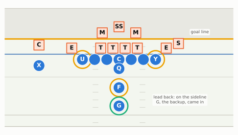
Reading the diagrams: offense is blue circles (X and Z wide receivers; Y and U tight ends, ringed in gold; F a fullback; Q quarterback; R running back); defense is outlined squares. Solid arrows are routes and runs, short arrows ending in a bar are blocks, dashed lines defenders’ movements. The dark blue line is the line of scrimmage. The charts come from nflverse data; the notes under each one say which seasons and filters it uses.

Outputs and inputs: why the box score misleads

A fantasy point is the end of a chain. For a wide receiver, the chain runs like this: his team runs a certain number of plays (pace); some fraction of them are passes (the play-caller’s tendency, adjusted by the score); on some of those passes he is on the field and running a route rather than blocking or standing on the sideline (route participation); on some of those routes the ball is thrown to him (target share), some of them deep (air-yards share); and on some of those targets he catches the ball, gains yards and, now and then, scores. Every link before the catch is mostly usage, and usage is set by people: the coordinator who designs the plays, the play-caller who chooses them on game day, and the quarterback who decides where the ball goes. The links after it are mostly efficiency, which belongs to the player, plus a large dose of luck.

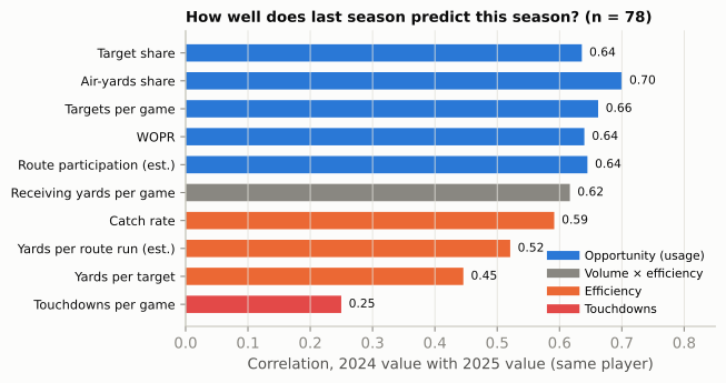
The reason to care about the difference is that the two halves behave very differently over time. The next figure takes every wide receiver and tight end with at least 50 targets in both 2024 and 2025 and asks a simple question of each statistic: if you knew a player’s 2024 number, how well would it predict his 2025 number?

def stab_frame(u):
    u = u[u.pos.isin(["WR", "TE"])].copy()
    u["tpg"], u["ypg"] = u.tgt / u.games, u.yds / u.games
    u["ypt"], u["tdpg"], u["catch"] = u.yds / u.tgt, u.td / u.games, u.rec / u.tgt
    u = u[u.tgt >= 50]
    return u.loc[u.groupby("pid").tgt.idxmax()].set_index("pid")


STAB = stab_frame(U24).join(stab_frame(U25), lsuffix="_24", rsuffix="_25", how="inner")
METRICS = [("tgt_share", "Target share", "use"), ("ay_share", "Air-yards share", "use"),
           ("tpg", "Targets per game", "use"), ("wopr", "WOPR", "use"),
           ("route_part", "Route participation (est.)", "use"),
           ("ypg", "Receiving yards per game", "mix"), ("catch", "Catch rate", "eff"),
           ("yprr", "Yards per route run (est.)", "eff"), ("ypt", "Yards per target", "eff"),
           ("tdpg", "Touchdowns per game", "td")]
vals = [(lab, STAB[f"{k}_24"].corr(STAB[f"{k}_25"]), grp) for k, lab, grp in METRICS]
COLORS = {"use": style.OFFENSE, "mix": style.MUTED, "eff": style.DEFENSE, "td": style.SERIES[7]}
fig, ax = plt.subplots(figsize=(6.4, 3.6))
for i, (lab, v, grp) in enumerate(vals[::-1]):
    ax.barh(i, v, color=COLORS[grp], height=0.62)
    ax.text(v + 0.012, i, f"{v:.2f}", va="center", fontsize=8, color=style.INK)
ax.set_yticks(range(len(vals)))
ax.set_yticklabels([v[0] for v in vals[::-1]], fontsize=8.5, color=style.INK)
ax.set_xlim(0, 0.85)
ax.set_xlabel("Correlation, 2024 value with 2025 value (same player)")
ax.grid(axis="y", visible=False)
ax.legend(handles=[Line2D([], [], color=COLORS[g], lw=6, label=l) for g, l in
                   [("use", "Opportunity (usage)"), ("mix", "Volume × efficiency"), ("eff", "Efficiency"),
                    ("td", "Touchdowns")]],
          loc="lower right", fontsize=8)
ax.set_title(f"How well does last season predict this season? (n = {len(STAB)})", fontsize=10)
plt.show()

Figure 73.1: Usage repeats; touchdowns don’t. Each bar is the correlation between a player’s 2024 and 2025 value of the statistic, for the 78 wide receivers and tight ends with 50 or more targets in both regular seasons (a player who changed teams counts with the team where he drew more targets). A correlation of 1 would mean the 2024 number predicts 2025 perfectly; 0, not at all. Blue bars measure opportunity, orange bars what the player did with each chance, the grey bar a mix of the two (yards per game is volume times efficiency), the red bar touchdowns. With 78 players, a correlation is uncertain by roughly ±0.08, so bars within about 0.1 of each other are not really different. Only players who kept a 50-target role in both seasons are included, so players who lost their role are missing. Route participation and yards per route run are estimated from on-field dropbacks (see the note on where route counts come from). Data: nflverse play-by-play and participation, this book’s calculation.

The opportunity numbers (target share, air-yards share, targets per game, WOPR, route participation) all correlate at about 0.64 to 0.70 from one season to the next. Be careful about what the chart does not say. Receiving yards per game (0.62) is almost as sticky, but it isn’t a pure efficiency number: it is volume times efficiency, so it inherits most of its stability from the volume. Catch rate (0.59) is sticky because it is partly a role too: a slot receiver who runs short routes catches a high share of his targets every year, and a deep threat a low one. The numbers that really wobble are the per-chance ones. Yards per target sits near 0.45, and touchdowns per game, the statistic that swings a fantasy week more than any other, correlate at only 0.25.

In plain terms, a receiver’s share of his team’s targets is mostly a fact about his role, and his role is decided before the season by the scheme, the depth chart and the quarterback’s trust. Whether a given target turns into a 40-yard catch or a touchdown depends on the coverage, the throw, the defender’s hand and a dozen things that don’t repeat. One honest caveat: the chart includes only receivers who kept a real role in both seasons, the survivors. A player who lost his job isn’t in it, so treat these correlations as “if the role holds”, which is exactly the question a scheme change raises.²

ImportantWhy it exists

Usage stats exist because fantasy players and analysts kept being fooled by box scores. A season of touchdowns makes a player look like a star; a season of near-misses makes an equally used player look ordinary. The next season, the touchdowns are dealt out again more or less at random, while the opportunity that produced them carries over. Reading usage is the habit of pricing a player on the part of his production that will repeat. The trade-off: usage tells you about the chances, not the talent. A player who gets the ball constantly and does nothing with it will eventually lose the role, so the efficiency numbers still matter. They are just slower to trust.

NoteMadden vs. real life

In Madden, a player’s ratings drive what he does on the field: a 95-overall receiver gets open and makes plays. In a real offense, the ball goes where the play was designed to send it, read by the quarterback in the order the play-caller drew it. A great receiver in a run-first offense that rotates its receivers can finish behind an average one in a pass-first offense that never takes him off the field. The talent is the same; the opportunity is not, and opportunity is drawn on the play-caller’s call sheet, not in the player’s ratings.

Receivers: from snaps to routes to targets

Being on the field is not the same as running a route

Start with the first filter. A player can’t catch a pass on a play he isn’t in for, so the first number to check is snap share: the share of the team’s offensive plays on which he is on the field, published by the league in its official snap counts (free in nflverse as load_snap_counts(), from Pro Football Reference). A team’s top two wide receivers usually play 85-95% of the snaps; a third receiver might play 60-80%, and his number depends on how often the team uses three-receiver sets.

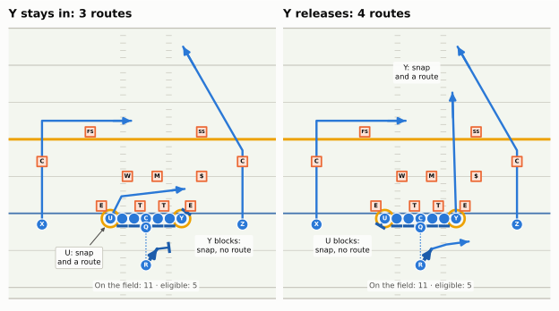
Snap share has a blind spot, and the tight end shows it best. The two-jobs figure draws the same 12 personnel formation twice.

def jobs_play(y_routes):
    off = line5() + [O("QB", "QB", -1.9, 0, "Q"), O("RB", "RB", -7.0, 0, "R"),
                     O("Y", "TE", -0.7, 4.8, "Y"), O("U", "TE", -0.7, -4.8, "U"),
                     O("X", "WR", -1.5, -14.0, "X"), O("Z", "WR", -1.5, 13.0, "Z")]
    dfn = [D("SDE", "DE", 1.0, 6.0, "E"), D("SDT", "DT", 1.0, 2.4, "T"), D("WDT", "DT", 1.0, -0.8, "T"),
           D("WDE", "DE", 1.0, -6.0, "E"), D("MIKE", "MIKE", 5.0, 1.5, "M"), D("WILL", "WILL", 5.0, -2.5, "W"),
           D("NB", "NB", 5.0, 7.5, "$"), D("LCB", "CB", 7.0, -14.0, "C"), D("RCB", "CB", 7.0, 13.0, "C"),
           D("FS", "FS", 11.0, -7.5, "FS"), D("SS", "SS", 11.0, 7.5, "SS")]
    p = Play(off, dfn, los=40, to_go=10)
    for k, t in [("LT", "WDE"), ("LG", "WDT"), ("C", "WDT"), ("RG", "SDT"), ("RT", "SDT")]:
        p.block(k, pts=[(-1.0, 0.0)])
    p.dropback(5.0)
    p.route("X", r.dig(14))
    p.route("Z", r.post(10))
    if y_routes:
        p.route("Y", r.seam(17))
        p.block("U", pts=[(-1.0, -0.6)])
        p.run("RB", [(2.2, 1.5)], speed=4.0)                       # the run fake
        p.route("RB", r.flat(depth=1.0, width=5), side=1, delay=0.5)  # check for a blitzer, then the flat
    else:
        p.block("Y", target="SDE")
        p.route("U", r.drag(3, 10))
        p.run("RB", [(2.2, 1.5)], speed=4.0)                       # the run fake
        p.block("RB", pts=[(0.2, 1.6)])                            # then sets up to protect
    p.highlight("Y", "U", color=TE_RING)
    return p


fig, axes = plt.subplots(1, 2, figsize=(6.6, 5.6))
for ax, y_routes, ttl in [(axes[0], False, "Y stays in: 3 routes"), (axes[1], True, "Y releases: 4 routes")]:
    p = jobs_play(y_routes)
    fld = p.draw(ax=ax, lateral=(-18, 17), window=(-11.5, 25), width_in=3.3, title=False)
    no_numbers(ax)
    ax.set_title(ttl, fontsize=9.5, loc="left", color=style.INK, fontweight="bold")
    if y_routes:
        say(fld, p, "U blocks:\nsnap, no route", (-4.4, -10.5), fs=6.3)
        say(fld, p, "Y: snap\nand a route", (19.0, -0.5), fs=6.3)
    else:
        say(fld, p, "Y blocks:\nsnap, no route", (-4.4, 10.5), fs=6.3)
        pointer(fld, p, "U: snap\nand a route", (-6.0, -9.0), (-1.0, -4.8), fs=6.3)
    say(fld, p, "On the field: 11 · eligible: 5", (-9.8, 0), fs=6.3, color=style.INK_2)
fig.tight_layout(w_pad=0.6)
plt.show()

Figure 73.2: One snap, two jobs (illustrative play-action passes from 12 personnel, under center). Both tight ends (gold rings) are on the field for both plays, so both get a snap in the official count. Left: a max-protection play-action shot. Y stays in to block the defensive end and the running back fakes the run and then protects, so seven men block four rushers and buy time for Z’s post and X’s dig; only three players run routes (X, Z and U on a drag underneath). The call itself takes Y out of the route count. Right: the same formation, but U stays in and Y runs up the seam while the back releases to the flat after checking for a blitzer, so four players run routes. Snap share can’t tell these plays apart. Routes charted from film can; the on-field estimate used in this chapter’s later charts can’t either (both tight ends are on the field in both pictures), which is why that estimate is an upper bound for tight ends.

In both pictures the two tight ends play the snap, so their snap counts are identical. In one of them Y is a blocker who never had a chance to catch the ball; in the other he is a receiver running up the seam. The left-hand call is a max-protect shot: the play-caller kept seven men in to buy time for two deep routes, and the price is the tight end’s route. Some calls take a tight end out of the pattern by design, and a play-caller who loves them is a bad landlord for a fantasy tight end. Over a season, a tight end who stays in to block on a third of his team’s dropbacks has a third fewer chances to be targeted than one who goes out every time. The same is true of a running back who stays in to protect the quarterback, a job called pass protection, or who chips a pass rusher before releasing late.

That is what route participation measures: the share of the team’s dropbacks (pass plays, including sacks and scrambles) on which a player runs a route. For a team’s top wide receivers it is usually above 85%, because a wide receiver almost never stays in to block on a pass play. (He still loses a few: on a screen to someone else he blocks for the ball carrier, and on some RPOs he blocks for the run half of the play while the quarterback throws to someone else. That, plus rest snaps, is why even a number-one receiver sits around 90-95%, not 100%.) For tight ends and backs it is where the real information is: two tight ends with the same snap share can have route participation of 50% and 85%, and only the second is a fantasy tight end.

NoteGo deeper: where route counts come from

Routes are not in the official play-by-play. Pro Football Focus (PFF) and FTN count them by watching film of every play, and sell the results. The free nflverse participation data tells you who was on the field for each play, but not who ran a route. This chapter therefore estimates route participation as the share of a team’s dropbacks on which a player was on the field. For wide receivers the estimate is close to the true figure; for tight ends and backs it overstates routes by however often they stayed in to block. When this chapter says “route participation (est.)”, that is the measure. Treat it as an upper bound for anyone who blocks.

Target share: how much of the passing game is aimed at him

A target is a pass thrown to an intended receiver, caught or not. Target share is a player’s targets divided by his team’s targets in the games he played. It is the single most useful receiving number, for two reasons. First, it is a share, so it strips out how much the team throws: 25% of a pass-heavy team’s targets and 25% of a run-heavy team’s targets describe the same role in two different amounts of work. Second, it is a role, and roles are designed. Play-callers feature a receiver in three main ways. They move his alignment (slot, boundary, motion) to get him the best leverage and the matchup they want. They build pre-snap “alerts” to him, so the quarterback throws his way whenever the defense leaves him one-on-one. And they manufacture touches: screens, quick throws and jet or orbit pitches that put the ball in his hands without a read at all. (Simply “making him the first read” is a smaller lever than it sounds, because progressions depend on the coverage: the first read against one coverage is often not the first read against another.) Mike McDaniel’s Miami offenses are the textbook case: built around Tyreek Hill’s and Jaylen Waddle’s speed with motion and quick touches, they aimed about 30% of their targets at Hill and about another 20% at Waddle in both 2022 and 2023.³

That gives target share two layers, and the difference matters later in this chapter. A genuine number-one receiver’s share is mostly his: talent and the quarterback’s trust earn it, and it tends to follow him from season to season (the 0.64 in the chart above). But how a team’s targets split by position, between wide receivers, tight ends and backs, is largely the play-caller’s fingerprint, and it moves when the play-caller does. A new coordinator who feeds his tight end has to take those targets from somebody, usually the second and third receivers first.

In 2025 a typical team’s leading receiver drew about 23% of its targets in the games he played; the true “alpha” receivers (fantasy slang for a team’s dominant number-one target) were near or above 30%. Seattle’s Jaxon Smith-Njigba, the 2025 Offensive Player of the Year, drew 36%, the highest share of any player with a full season, and Detroit’s Amon-Ra St. Brown and Cincinnati’s Ja’Marr Chase each drew about 31-32%. A player in the 15-20% range is a secondary option; his weekly output depends on how the defense plays the primary one.

Air-yards share and WOPR: not all targets are equal

A 2-yard pass in the flat and a 30-yard throw down the sideline each count as one target, but they are not worth the same. The deep one, caught, is worth far more yards and points. Air-yards share captures that: add up the air yards of every pass thrown to the player (how far past the line of scrimmage each traveled in the air) and divide by the team’s total. A slot receiver who catches short passes can have a big target share and a modest air-yards share; a deep threat can have the reverse.

Josh Hermsmeyer, an analyst who built the air-yards site airyards.com and later wrote for FiveThirtyEight, combined the two into one number: WOPR, the weighted opportunity rating.⁴

\[\text{WOPR} = 1.5 \times \text{target share} + 0.7 \times \text{air-yards share}\]

Target share gets the bigger weight, and the logic is that a target is a chance at a reception, yards and a touchdown all at once, while air yards add the size of the chance. As a scale, a WOPR of about 0.7 or more marks a team’s clear number-one target; 0.4 to 0.5 is a typical number two. In 2025 Smith-Njigba’s was about 0.89 (a 36% target share and half of Seattle’s air yards), the highest in the league. Carolina’s Tetairoa McMillan, the Offensive Rookie of the Year, drew a quarter of the Panthers’ targets and about 43% of their air yards for a WOPR near 0.68, among the league’s top ten: a rookie who was the deep, contested-catch target from his first game.

What does WOPR add, if it is no stickier than target share (0.64 and 0.64 in the chart above)? Less than its fame suggests, for predicting points. In this book’s 78-receiver sample, a player’s 2024 WOPR and his 2024 target share predict his 2025 fantasy points per game (in PPR scoring, explained below) equally well (correlations of about 0.58 and 0.57). WOPR’s real use is description: two receivers with the same 22% target share are different players if one has 35% of the air yards and the other 12%, and WOPR folds that into the same number. Use it to see the shape of a role, not as a better crystal ball.⁵

Yards per route run: efficiency with the right denominator

Opportunity is half the story; the other half is what a player does with it. The classic efficiency numbers (catch rate, yards per catch, yards per target) all divide by something the player earned only after he got open. Yards per route run (YPRR) divides receiving yards by the number of routes the player ran, every chance he had to get open, whether or not the ball came his way. It rewards both halves: a receiver who earns targets and gains yards on them scores well, and one who runs a hundred routes for nothing scores badly. Around 1.5 is typical for a regular NFL wide receiver; 2.0 is very good; 2.5 or more is elite.

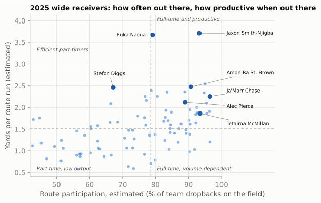
The two numbers together, how often a receiver is out there and how productive he is when he is, form a simple map.

W25 = U25[(U25.pos == "WR") & (U25.db_on >= 250)].copy()
mx, my = W25.route_part.median(), W25.yprr.median()
fig, ax = plt.subplots(figsize=(6.4, 4.3))
ax.scatter(W25.route_part * 100, W25.yprr, s=18, color=style.OFFENSE, alpha=0.55, lw=0)
ax.axvline(mx * 100, color=GREY, lw=0.9, ls=(0, (4, 3)))
ax.axhline(my, color=GREY, lw=0.9, ls=(0, (4, 3)))
# label positions in data coordinates; the cluster of full-time receivers is labelled in the right margin
LABEL = {"Jaxon Smith-Njigba": (101.5, 3.71, "left"), "Puka Nacua": (77.0, 3.67, "right"),
         "Stefon Diggs": (66.0, 2.78, "center"),
         "Amon-Ra St. Brown": (101.5, 2.80, "left"), "Ja'Marr Chase": (101.5, 2.38, "left"),
         "Alec Pierce": (101.5, 2.02, "left"), "Tetairoa McMillan": (101.5, 1.62, "left")}
for nm, (tx, ty, ha) in LABEL.items():
    row = W25[W25.name == nm]
    if row.empty:
        continue
    x, y = float(row.route_part.iloc[0] * 100), float(row.yprr.iloc[0])
    ax.scatter([x], [y], s=34, color=style.OFFENSE_DARK, zorder=4)
    ax.annotate(nm, (x, y), xytext=(tx, ty), fontsize=7.2, ha=ha, va="center", color=style.INK,
                arrowprops=dict(arrowstyle="-", color=GREY, lw=0.6, shrinkA=1, shrinkB=3))
for txt, xy, ha in [("Efficient part-timers", (44, 3.3), "left"), ("Full-time and productive", (80.5, 4.0), "left"),
                    ("Full-time, volume-dependent", (80.5, 0.55), "left"),
                    ("Part-time, low output", (44, 0.55), "left")]:
    ax.text(*xy, txt, fontsize=7.5, color=style.INK_2, ha=ha, style="italic")
ax.set_xlim(42, 116)
ax.set_xticks(range(50, 101, 10))
ax.spines["bottom"].set_bounds(42, 100)
ax.set_ylim(0.4, 4.15)
ax.set_xlabel("Route participation, estimated (% of team dropbacks on the field)")
ax.set_ylabel("Yards per route run (estimated)")
ax.set_title("2025 wide receivers: how often out there, how productive when out there", fontsize=10)
plt.show()

Figure 73.3: Route participation against yards per route run, 2025 wide receivers with 250 or more dropbacks on the field (estimated from participation data: the share of the team’s dropbacks, in games he played, on which he was on the field; and receiving yards divided by those dropbacks). Dashed lines are the medians (about 79% and 1.5). Top right: full-time players who produce on every route, the safest fantasy receivers. Top left: efficient part-timers, whose value rises if their role grows. Bottom right: full-time players whose production per route is modest; they depend on volume. Bottom left: part-timers who don’t produce much when they are out there, the waiver-wire pool. Regular seasons only.

Smith-Njigba and the Rams’ Puka Nacua sit alone at the top, at about 3.7 yards per route, numbers that happen a few times a decade. Nacua’s dot sits on the median line for participation, which looks odd for a star. It is scheme, not demotion: the 2025 Rams used 13 personnel (three tight ends and one receiver) on about a fifth of their dropbacks, and Nacua was on the field for fewer than half of those; he also left one October game early and missed the next. On the Rams’ three-receiver plays he was out there about 85% of the time.⁶ The more interesting dots for fantasy are the ones in the top left: New England’s Stefon Diggs produced almost 2.5 yards per route while on the field for only about two-thirds of the Patriots’ dropbacks. A part-timer that productive is the cheapest kind of upside: if an injury or a new coordinator turns him into a full-timer, his volume rises by a third and his efficiency doesn’t have to improve at all. The bottom right holds the opposite profile, full-time receivers who are useful only as long as the volume keeps coming.

CautionCommon misconception

“He had 9 catches for 140 yards, so he’s the number-one receiver now.” One big game is mostly efficiency, and efficiency is the noisy half. Check the usage behind it: was he on the field for more routes than usual, and did his target share actually rise? If he ran his usual 60% of routes and three long passes happened to find him, nothing about his role changed. If his route participation jumped from 60% to 90% because the starter went down, the role changed, and that is worth acting on even if the box score was quiet.

Running backs: snaps, carries, routes and the goal line

A running back’s usage has more parts than a receiver’s, because he does more jobs. Read it in four pieces.

1. Snap share. Very few backs play every down now. A true “bell cow” (one back who plays nearly every down and gets nearly every carry) plays 75-85% of the snaps; most backfields split, with an early-down back and a passing-down back sharing 50-60% each.
2. Share of the carries. How many of the team’s runs he gets. This depends on the team’s run rate as well as his role, so check both.
3. Routes and targets. A back who runs routes on third down and in the two-minute drill gets targets that a pure runner never sees, and in PPR scoring (below) each catch is worth a point. Backs run routes on far fewer dropbacks than receivers, because they often stay in to protect, and protection is the gate to this role: the most common reason a talented receiving back (often a rookie) doesn’t get third-down snaps is that the staff doesn’t trust him to pick up a blitzer (Pass Protection). Not all back targets are equal, either. Designed targets (screens, and option or angle routes built to get the back the ball, the way the Shanahan tree used Christian McCaffrey) are worth more than check-downs thrown only when everything else is covered, and they travel with the play-caller who draws them.
4. Red-zone share. His share of the team’s carries and targets inside the opponent’s 20-yard line (the red zone), and above all inside the 5. Most touchdowns are scored from close range, so the goal-line role decides a back’s touchdown total more than his talent does.

The last one is where scheme hides the most fantasy value, and two recent backfields show it from both directions.

def chances(season, team, max_yl):
    d = PLAYS[(PLAYS.season == season) & (PLAYS.posteam == team) & (PLAYS.yardline_100 <= max_yl) & (PLAYS.qb_kneel != 1)]
    who = np.where(d.play_type == "run", d.rusher_player_id, d.receiver_player_id)
    ok = pd.notna(who)
    td = (d.rush_touchdown + d.pass_touchdown).values[ok]
    return pd.DataFrame({"pid": who[ok], "td": td})


def share(season, team, max_yl, pid):
    c = chances(season, team, max_yl)
    return 100 * (c.pid == pid).mean()


def pid_of(name):
    return PEOPLE.loc[PEOPLE.display_name == name, "gsis_id"].iloc[0]


SNAPS = NFL.load_snap_counts([2024, 2025]).to_pandas()
SNAPS = SNAPS[SNAPS.game_type == "REG"]


def snap_share(season, name):
    return 100 * SNAPS[(SNAPS.season == season) & (SNAPS.player == name)].offense_pct.mean()


def carry_share(season, team, pid):
    d = PLAYS[(PLAYS.season == season) & (PLAYS.posteam == team) & (PLAYS.play_type == "run") & (PLAYS.qb_kneel != 1)]
    return 100 * (d.rusher_player_id == pid).mean()


fig, axes = plt.subplots(1, 2, figsize=(6.6, 3.0), gridspec_kw=dict(width_ratios=[1.35, 1]))
ax = axes[0]
sea = [("Kenneth Walker III", style.OFFENSE), ("Zach Charbonnet", style.DEFENSE)]
SEA_RUSH_TD = PLAYS[(PLAYS.season == 2025) & (PLAYS.posteam == "SEA") & (PLAYS.rush_touchdown == 1)].rusher_player_id.value_counts()
cats = ["Snaps", "Carries", "Red-zone\nchances", "Inside-5\nchances"]
for j, (nm, col) in enumerate(sea):
    pid = pid_of(nm)
    v = [snap_share(2025, nm), carry_share(2025, "SEA", pid), share(2025, "SEA", 20, pid), share(2025, "SEA", 5, pid)]
    xs = np.arange(len(cats)) + (j - 0.5) * 0.38
    ax.bar(xs, v, width=0.36, color=col, label=f"{nm}: {int(SEA_RUSH_TD.get(pid, 0))} rush TD")
    for x, val in zip(xs, v):
        ax.text(x, val + 1.2, f"{val:.0f}", ha="center", fontsize=7, color=style.INK)
ax.set_xticks(range(len(cats)))
ax.set_xticklabels(cats, fontsize=7.5)
ax.set_ylim(0, 74)
ax.set_ylabel("Share of Seattle's total (%)")
ax.grid(axis="x", visible=False)
ax.legend(fontsize=7, loc="upper left", ncol=1)
ax.set_title("Seattle 2025: same snaps, different jobs", fontsize=9)

ax = axes[1]
hurts, barkley = pid_of("Jalen Hurts"), pid_of("Saquon Barkley")
c2 = chances(2024, "PHI", 2)
groups = [("Chances\ninside the 2", lambda c, p: (c.pid == p).sum()),
          ("TDs from\ninside the 2", lambda c, p: c[(c.pid == p)].td.sum())]
for j, (nm, pid, col) in enumerate([("Hurts (QB)", hurts, style.SERIES[2]), ("Barkley (RB)", barkley, style.OFFENSE)]):
    xs = np.arange(len(groups)) + (j - 0.5) * 0.38
    v = [f(c2, pid) for _, f in groups]
    ax.bar(xs, v, width=0.36, color=col, label=nm)
    for x, val in zip(xs, v):
        ax.text(x, val + 0.3, f"{val:.0f}", ha="center", fontsize=7, color=style.INK)
ax.set_xticks(range(len(groups)))
ax.set_xticklabels([g[0] for g in groups], fontsize=7.5)
ax.set_ylim(0, 21)
ax.set_ylabel("Plays")
ax.grid(axis="x", visible=False)
ax.legend(fontsize=7, loc="upper right")
ax.set_title("Philadelphia 2024: the tush push", fontsize=9)
fig.tight_layout(w_pad=1.2)
plt.show()

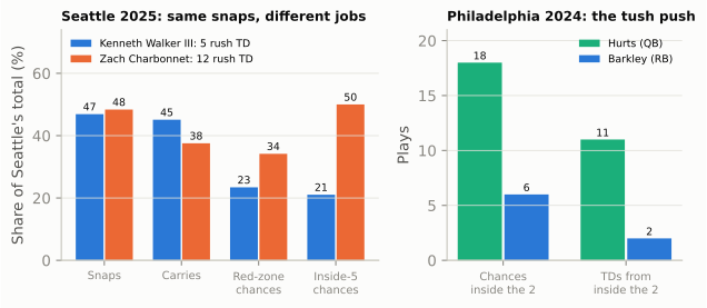
Figure 73.4: Who gets the ball near the goal line. Left: Seattle’s 2025 backfield. Kenneth Walker III and Zach Charbonnet were on the field for about the same share of snaps, and Walker got more of the carries, but Charbonnet got about half of the team’s chances inside the 5-yard line, and the rushing touchdowns (in the legend) followed the goal-line job, not the carries. Right: Philadelphia, 2024, inside the 2-yard line, where the ball went to the quarterback rather than the 2,005-yard running back (the film room below tells the story). ‘Chances’ are carries plus targets; snap shares are game averages from the official counts. Data: nflverse play-by-play and snap counts (Pro Football Reference), regular seasons.

Seattle’s split is the classic two-back design. Walker was the early-down runner who got more of the carries between the 20s (the long middle of the field, between the two 20-yard lines); Charbonnet, a capable short-yardage runner, was the back the coaches trusted near the goal line. Walker’s 221 carries brought 5 rushing touchdowns; Charbonnet’s 184 brought 12, and in standard scoring Charbonnet out-scored him for the season. The snap share said “even split.” The red-zone share said who would score.

That is the backup from this chapter’s opening. A back who plays 14 snaps and scores twice from the 1 is either lucky or holding a job, and the box score can’t tell you which. Check who was in the game every time the team got inside the 5. If it was him each time, the touchdowns will keep coming even if his snap count never grows; if it was a different back each time, they were a coin flip that landed his way.

NoteFilm room: Eagles 2024 — Saquon Barkley’s 2,005 yards

Philadelphia signed Saquon Barkley as a free agent from the Giants in March 2024. Fantasy drafters were wary: he was 27, coming off a down year behind a poor line, and joining a team whose quarterback scored short touchdowns himself. In July his consensus average draft position (ADP, the pick at which drafters typically took him, in half-PPR scoring, which gives half a point per catch; both are explained below) was about the 17th pick, the middle of the second round in a typical league and the sixth running back off the board. That was the lowest of his career.⁷

What he joined was a scheme built to feed a back. The Eagles’ line was the best-funded in football (see Building a Roster and the Eagles case study), and the play-callers leaned on it: in neutral situations the 2024 Eagles passed about 9 percentage points less often than an average team in the same situations, the third-lowest PROE in the league. They also led often, and a team protecting a lead runs. Barkley took 58% of the Eagles’ runs and played about three-quarters of the snaps, and he finished with 2,005 rushing yards on 345 carries and 13 rushing touchdowns in 16 games, sitting out Week 18 with the Eagles already locked into the NFC’s No. 2 seed.⁸

Now look at what he didn’t get. His 43 targets were modest for a lead back, because Philadelphia’s passing game ran through A.J. Brown and DeVonta Smith. And at the goal line the ball went to the quarterback: the Eagles’ tush push, a quarterback sneak with teammates pushing from behind (built in full in Red Zone, Goal Line, and Short Yardage), was so reliable that inside the 2-yard line Hurts got 18 chances to Barkley’s 6 and scored 11 times to Barkley’s 2 (the right panel of the goal-line chart). Those sneaks also shaded his red-zone share: by taking the shortest, surest carries off his plate, they left him the chances that start farther out and convert less often, so even his healthy-looking share inside the 20 overstated his touchdown odds. A back with 2,005 yards finished the season first among running backs in standard scoring but second in PPR, behind Detroit’s Jahmyr Gibbs, who ran less but caught more.

What to notice: every input that made the season was visible before it started: a run-first play-caller, an elite line, a team expected to lead. So was the one that capped it, the quarterback’s goal-line role. The market priced the worry (the goal line) and underpriced the volume.

The same goal-line play has a winner, and he is the quarterback. Standard fantasy scoring pays six points for a rushing touchdown but usually four for a passing one, and a point for every 10 rushing yards against one per 25 passing yards. A quarterback who runs, and above all one who scores on sneaks, collects the most valuable touches on the field. Hurts threw for only 2,903 yards in 2024, but his 14 rushing touchdowns kept him the eighth-best fantasy quarterback in standard scoring despite missing two games.⁹ When you read a team’s goal-line usage, read it for the quarterback too: the tush push is a running back’s tax and a quarterback’s dividend.

The tight end in 12 personnel: blocker or receiver?

No position’s fantasy value depends more on scheme than the tight end’s, because no position’s job varies more. In 12 personnel (one back, two tight ends, two receivers) the two tight ends usually have different jobs. One is the in-line tight end, attached to the end of the line, whose first job is blocking; the other is often the move tight end, who lines up in the slot, as a wing or in the backfield and is a receiver first. Offenses used 12 personnel on 24.4% of plays in 2025, a decade high in this book’s count, and fewer than three wide receivers on 41.7% of plays by Next Gen Stats’ count.¹⁰ More tight end snaps do not mean more tight end routes: the second tight end in a heavy set is often there to block, which is exactly why the offense put him there instead of a third receiver.

So for a tight end, read three numbers in order.

• Route participation, not snap share. A tight end who runs a route on 80% or more of dropbacks is used as a receiver; one at 50-60% is a blocker who sometimes goes out. Fantasy points live almost entirely in the first group. In 2025, by this chapter’s on-field estimate, Arizona’s Trey McBride was out there on about 94% of the Cardinals’ dropbacks and Detroit’s Sam LaPorta on about 92% (true route rates are a little lower, since both sometimes block); the Rams, who rotated tight ends through their three-tight-end package, had Tyler Higbee and Colby Parkinson near 56-59%, before subtracting the snaps they spent blocking.¹¹
• Target share among route runners. Some offenses aim the passing game at the tight end. In 2025 Arizona threw 35% of its targets to tight ends, the most in the league, and Trey McBride alone drew 27% of the Cardinals’ targets, more than any wide receiver on the team.
• Red-zone usage. Tight ends are big targets in tight spaces, and some offenses build their goal-line pass plays around them. A tight end with few yards but a steady red-zone role is a touchdown bet, with the noise that implies.

Back to the tight end from the opening, on the field for 52 of 61 snaps with one catch. The first question is not whether he is good but how many of those 52 snaps were routes. If he blocked on half of them, the one catch is about what that role produces, and no amount of patience will fix it. If he ran a route on 40-plus and saw only two or three targets, the role is right and the targets are noise worth waiting out.

The Arizona number matters for 2026, because the coordinator who built that offense now calls plays in Detroit. We’ll come back to him.

Volume: how much the team throws, how fast, and why the score changes it

Shares tell you a player’s slice. Volume is the size of the pie, and it is set at the team level by three things: how pass-happy the play-caller is, how many plays the offense runs, and the score.

Pass rate over expected

PROE measures the first. It compares how often a team passes to how often an average team would pass in the same down, distance, field position, score and time, so it isolates the play-caller’s taste from the situations he was handed. The next figure shows why it matters for fantasy, and what it does not do.

T25 = TEAMS.xs(2025).copy()
top = U25.sort_values("tgt", ascending=False).groupby("posteam").head(1).set_index("posteam")
T25["top_share"] = top.tgt_share * 100
T25["top_name"] = top.name
fig, axes = plt.subplots(1, 2, figsize=(6.6, 3.4), sharex=True)
for ax, col, ylab, ttl in [(axes[0], "top_share", "Top target's share of team targets (%)", "The share"),
                           (axes[1], "targets_pg", "Team targets per game", "The volume")]:
    ax.scatter(T25.proe, T25[col], s=20, color=style.OFFENSE, alpha=0.75, lw=0)
    b, a = np.polyfit(T25.proe, T25[col], 1)
    xx = np.array([-13, 7])
    ax.plot(xx, a + b * xx, color=style.INK_2, lw=1.0, ls=(0, (4, 3)))
    rho = T25.proe.corr(T25[col])
    ax.set_title(f"{ttl}  (r = {rho:.2f})", fontsize=9)
    ax.set_ylabel(ylab, fontsize=8)
    ax.set_xlabel("Neutral-situation PROE (percentage points)", fontsize=8)
for tm in ["NYJ", "BAL", "SEA", "ARI", "CIN", "LA", "DET"]:
    for ax, col in [(axes[0], "top_share"), (axes[1], "targets_pg")]:
        x, y = T25.loc[tm, "proe"], T25.loc[tm, col]
        off = (-4, -9) if (tm == "SEA" and col == "targets_pg") else (3, 3)
        ax.annotate(tm, (x, y), xytext=off, textcoords="offset points", fontsize=6.5, color=style.INK_2)
axes[0].set_ylim(15, 40)
fig.tight_layout(w_pad=1.0)
plt.show()

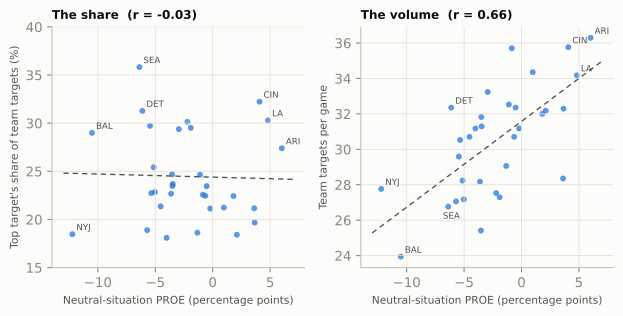
Figure 73.5: PROE moves the volume, not the share. Each dot is one team in 2025. Left: the share of the team’s targets that went to its most-targeted player, against the team’s neutral-situation PROE. There is no relationship (correlation about 0): how pass-heavy a team is says nothing about how concentrated its targets are. Right: the team’s targets per game against the same PROE. Here the relationship is strong (correlation about 0.66): pass-heavy teams throw more passes, so a given target share is worth more targets. PROE here is the neutral-situation version from Tendencies (downs 1-3, win probability between 20% and 80%, outside the last two minutes of each half). Regular season.

The left panel is the reassuring one: a receiver’s slice doesn’t depend on whether his team likes to throw. Seattle (PROE about −6) and the Rams (about +5) both funneled their passing games through one receiver, while the Jets, the most run-heavy team in neutral situations, spread theirs thin. The right panel is the one that moves fantasy values. Arizona, the league’s most pass-happy team at about +6, threw about 36 targets a game; Baltimore, at about −10, threw about 24. The same 25% target share is 9 targets a game in Arizona and 6 in Baltimore, a 50% difference produced mostly by the play-caller’s taste, with game script (Arizona trailed a lot) and the quarterback’s legs (Lamar Jackson’s scrambles and designed runs are pass calls and run plays that never become targets) doing the rest.

That gives the basic volume equation for any receiver:

\[\text{targets per game} \approx \text{plays per game} \times \text{pass rate} \times \text{target rate} \times \text{target share}\]

where the pass rate is set by PROE plus the situations the team gets into, and the “target rate” (the share of pass plays that produce a target, rather than a sack, scramble or throwaway) is usually around 85-90%. A coordinator change moves the first three terms at a stroke: his pace, his pass rate, even how often his pass calls end in a target. It moves the last term more selectively. A clear number-one receiver’s share mostly comes with him (that is his role), but a play-caller with a different position split, say one who feeds his tight end, reshuffles the shares of everyone below the top.

Pace

Pace is the number of plays. In 2025 the slowest offenses (Miami, Minnesota and Las Vegas) ran about 55 plays a game; the fastest (Dallas and Chicago) ran about 64-65. Ten extra plays a game is roughly 15-18% more opportunity for every player on the offense, before anyone’s share changes. Pace has two sources: how quickly a team gets to the line and snaps the ball (its tempo, built in In-Game Adjustments and Tempo), and how many first downs it earns, since drives that keep moving produce more plays. A good defense helps too: an offense gets more possessions when its own defense gets off the field fast.

Game script

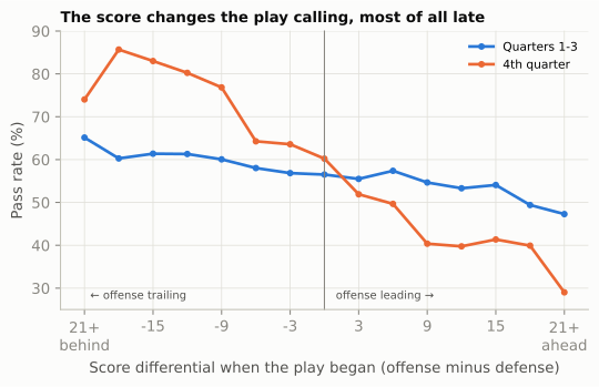
The score is the last term, and it is the one fantasy players talk about most. Game script is the way the score shapes play calling. A team ahead late runs the ball (the four-minute offense), which keeps the clock moving (an incomplete pass stops it), protects against turnovers and wears down a defense; a team behind throws, because it needs points fast and passes gain more per play. The effect is large enough to swamp a play-caller’s taste.

gs = PLAYS[(PLAYS.season == 2025) & (PLAYS.half_seconds_remaining > 120) & PLAYS.score_differential.notna()].copy()
gs["bin"] = (gs.score_differential.clip(-21, 21) / 3).round() * 3
gs["period"] = np.where(gs.qtr >= 4, "4th quarter", "Quarters 1-3")
gtab = gs.groupby(["period", "bin"])["pass"].mean().unstack(0) * 100
fig, ax = plt.subplots(figsize=(6.4, 3.4))
for col, c in [("Quarters 1-3", style.OFFENSE), ("4th quarter", style.DEFENSE)]:
    ax.plot(gtab.index, gtab[col], color=c, marker="o", ms=3.5, label=col)
ax.axvline(0, color=GREY, lw=0.8)
ax.text(-20.5, 27.5, "← offense trailing", fontsize=7.5, color=style.INK_2)
ax.text(1.0, 27.5, "offense leading →", fontsize=7.5, color=style.INK_2, ha="left")
ax.set_xlabel("Score differential when the play began (offense minus defense)")
ax.set_ylabel("Pass rate (%)")
ax.set_ylim(25, 90)
ax.set_xticks(range(-21, 22, 6))
ax.set_xticklabels(["21+\nbehind" if t == -21 else ("21+\nahead" if t == 21 else str(t)) for t in range(-21, 22, 6)])
ax.legend(fontsize=8, loc="upper right")
ax.set_title("The score changes the play calling, most of all late", fontsize=10)
plt.show()

Figure 73.6: Game script: how often teams passed at each score, 2025. Each point is the pass rate (dropbacks, including sacks and scrambles, as a share of plays) for plays with that score differential from the offense’s point of view, grouped in 3-point steps, with everything beyond 19 points pooled at the ends (‘21+’); the last two minutes of each half are excluded because the clock dominates them. In the first three quarters the line is fairly flat, from about 65% when far behind to about 47% when far ahead. In the fourth quarter it tilts sharply: about 80% when behind by two scores, about 40% or less when ahead by two scores. The fourth-quarter dip at the far left is not a mistake: down 20 or more late, the game is over (win probability under 2% on almost every such snap), and many teams stop chasing, run the clock out and rest starters. Regular season.

For fantasy, game script is why a receiver on a bad team can be a good pick (his team will trail, and trailing teams throw) and why a running back on a good team can be one (his team will lead, and leading teams run). It is also why one game’s usage can mislead: a running back who got 28 carries in a 31-3 win got them because of the score, not because his role grew, and the week his team trails he may get 11. When you read a weekly usage line, ask what the score was.

You can forecast the script before kickoff, and the tool is the betting market. A game’s point spread is the bookmakers’ estimate of the winning margin (“Chiefs −7” means Kansas City is expected to win by about seven), and the total (over/under) is their estimate of the combined points. Together they give each team an implied team total: half the total plus half the spread for the favorite, minus half the spread for the underdog. A −7 favorite in a game with a 45-point total is implied to score about 26 and allow about 19. For a whole season, the win totals posted before the season do the same job. In 2025 the spread did a decent job of predicting the script: teams favored by 7 or more led by about 4 points on an average snap, and teams that were underdogs by 7 or more trailed by about 8. Implied totals predicted actual points about as well (big favorites scored about 28 a game, big underdogs about 17).¹²

What the script changes is more specific than “trailing teams throw.” Those 2025 big favorites ran about 26 times a game and the big underdogs about 23, but both dropped back to pass about 35 times. The favorite’s extra snaps went to the ground, and its extra points went to whoever scores them. So for fantasy, a big spread is mainly a running-back and touchdown signal: the lead back of a heavy favorite gets more carries and more goal-line trips. For receivers, the bad-team bonus is real but smaller than people expect, because a team that trails all day also runs fewer plays and scores less. The cleanest usage numbers come from the stretches when the game was close, the same reason PROE is measured in neutral situations, and why analysts drop garbage time when they measure a team.

CautionCommon misconception

“Pass-heavy teams are always better for receivers.” Separate the team’s taste from its fate. Taste is PROE: how much the play-caller likes to throw when the game is close. It repeats, and it reliably raises volume. Fate is the score: a bad team that trails throws more late, but those targets depend on being behind, come in shorter bursts, and often come against a prevent defense that gives up short catches to protect the lead. They count for fantasy all the same, but they vanish the week the team keeps it close. Project a receiver’s volume from the taste first, then adjust for the likely fate using the betting lines.

Scoring formats and the market

Standard, half-PPR and PPR

Fantasy football began as a touchdown game. The first league, the Greater Oakland Professional Pigskin Prognosticators League, was dreamed up in 1962 by Bill Winkenbach, a limited partner in the Oakland Raiders, and held its first draft in 1963, with scoring based on touchdowns and kicks.¹³ As statistics became easy to collect, leagues added yards, and the scoring that most hosting sites called “standard” settled into one point per 10 rushing or receiving yards, six per touchdown, one per 25 passing yards and four per passing touchdown, minus two for an interception or a lost fumble (some sites take off only one for an interception).

Standard scoring had a problem: it made running backs who scored touchdowns far more valuable than anyone else, and it made a 9-catch, 70-yard day by a slot receiver worth less than a single 1-yard touchdown run. PPR (point per reception) scoring adds one point for every catch, and half-PPR adds half a point. It spread through serious leagues in the 2000s, and a version of it is now the default at the major hosting sites (full PPR at ESPN, half-PPR at Yahoo).¹⁴ The change is not cosmetic: it moves the whole market toward the players whose usage is receptions.

PS = NFL.load_player_stats([2025], summary_level="reg").to_pandas()
PICKS = {"RB": ["Christian McCaffrey", "Jonathan Taylor", "Kenny Gainwell", "Derrick Henry", "Zach Charbonnet"],
         "WR": ["Wan'Dale Robinson", "Justin Jefferson", "Stefon Diggs", "Tee Higgins", "Alec Pierce"]}
fig, axes = plt.subplots(1, 2, figsize=(6.6, 3.3), sharey=True)
for ax, (pos, names) in zip(axes, PICKS.items()):
    d = PS[PS.position == pos].copy()
    d["std"] = d.fantasy_points.rank(ascending=False, method="min")
    d["ppr"] = d.fantasy_points_ppr.rank(ascending=False, method="min")
    d["half"] = ((d.fantasy_points + d.fantasy_points_ppr) / 2).rank(ascending=False, method="min")
    d = d.set_index("player_display_name").loc[names].sort_values("ppr")
    for i, (nm, row) in enumerate(d.iterrows()):
        up = row.ppr < row["std"]
        col = style.OFFENSE if up else style.DEFENSE
        ax.plot([row["std"], row.ppr], [i, i], color=col, lw=2, zorder=2)
        ax.scatter([row["std"]], [i], s=36, facecolor=style.SURFACE, edgecolor=col, lw=1.4, zorder=3)
        ax.scatter([row.ppr], [i], s=36, color=col, zorder=3)
        ax.scatter([row.half], [i], s=60, marker="|", color=style.INK, lw=1.3, zorder=4)
        short = nm.split(" ")[-1] if nm != "Kenneth Walker III" else "Walker"
        ax.text(max(row["std"], row.ppr) + 2.0, i, f"{short}  {int(row['std'])} → {int(row.half)} → {int(row.ppr)}",
                va="center", fontsize=7, color=style.INK)
    ax.set_yticks([])
    ax.set_xlim(0, 52)
    ax.invert_yaxis()
    ax.grid(axis="y", visible=False)
    ax.set_xlabel(f"{pos} rank (1 = best)", fontsize=8)
    ax.set_title("Running backs" if pos == "RB" else "Wide receivers", fontsize=9)
fig.tight_layout(w_pad=0.8)
fig.legend(handles=[Line2D([], [], marker="o", ls="", mfc=style.SURFACE, mec=style.INK_2, label="Standard rank"),
                    Line2D([], [], marker="|", ls="", color=style.INK, ms=8, mew=1.3, label="Half-PPR rank"),
                    Line2D([], [], marker="o", ls="", color=style.INK_2, label="PPR rank"),
                    Line2D([], [], color=style.OFFENSE, lw=2, label="Better in PPR"),
                    Line2D([], [], color=style.DEFENSE, lw=2, label="Worse in PPR")],
           loc="upper center", bbox_to_anchor=(0.5, 0.0), ncol=5, fontsize=6.6, handletextpad=0.3, columnspacing=0.9)
plt.show()

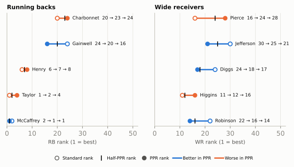
Figure 73.7: The same 2025 season under three scoring systems. Each line runs from a player’s position rank in standard scoring (open circle) through half-PPR (black tick) to PPR (filled circle); rank 1 is the best at his position, and the label reads standard → half-PPR → PPR. Players who catch a lot of short passes (Kenny Gainwell, a pass-catching back with 73 catches on only 114 carries; Wan’Dale Robinson, a 140-target slot receiver) climb as catches count for more. Touchdown-heavy or deep-ball players (Jonathan Taylor, 18 rushing touchdowns; Alec Pierce, a deep threat with 84 targets and 47 catches) fall. Half-PPR usually lands between the two, but not exactly halfway, because everyone else’s rank is moving too. Fantasy points as computed by nflverse (load_player_stats; half-PPR as the average of the two), regular season.

Read the format before you read the usage. In standard scoring, a back’s carries and goal-line role are nearly everything; in PPR, a back who runs routes on third down can out-score a back with twice his carries. In 2025 Pittsburgh’s Kenny Gainwell was the 24th-best running back in standard scoring and the 16th in PPR, a jump bought entirely with 73 catches. Indianapolis’s Jonathan Taylor went the other way: first in standard, fourth in PPR, because 18 rushing touchdowns count the same in both systems while his 46 catches counted for less than Christian McCaffrey’s 102. McCaffrey, the Comeback Player of the Year, was the only back who did both, and he finished first in PPR. Derrick Henry (16 rushing touchdowns, 15 catches) slid the same way as Taylor, and so did Zach Charbonnet, Seattle’s goal-line back from earlier in the chapter: his 12 touchdowns made him a useful standard-league back, and his 20 catches made him a marginal PPR one.

The receivers tell the same story from the other side. Justin Jefferson drew 141 targets and caught 84 passes but scored only twice, so he was the 30th receiver in standard scoring and the 21st in PPR; his catches propped him up while his touchdowns didn’t. Tee Higgins, with 11 touchdowns on 59 catches, went the opposite way, from 11th to 16th. Look back at the stability chart: catches and targets repeat, touchdowns mostly don’t, so a format that pays for catches is also a format that rewards the more predictable kind of production.

ADP: the market price

ADP (average draft position) is the average pick at which a player is taken across many drafts on a hosting site. It is the closest thing fantasy has to a market price, and it behaves like one: it aggregates thousands of opinions and reacts to news. It comes in two forms. Overall ADP is the pick number across all positions (Barkley’s 17 in 2024); positional ADP is the order within a position (“RB6”: the sixth running back taken). Positional ADP is what you compare with a player’s finish, which is also counted by position.

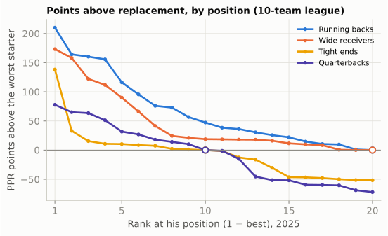
Overall ADP raises a question that connects straight back to Building a Roster. NFL teams treat running backs as cheap; fantasy drafters take them in the first round. Why does the same position sit at the bottom of one market and the top of the other? Because fantasy has its own version of positional value, and it comes from two things. First, fantasy scores touches and touchdowns, and a lead back gets more of both than anyone but the quarterback. Second, and more important, a player’s draft value is not his points but his points above replacement: what he scores beyond the best player you could get for free or late at the same lineup slot. In a 10-team league that starts one quarterback, two running backs, two receivers and a tight end, the baseline is roughly the 10th quarterback, the 20th running back, the 20th receiver and the 10th tight end, the worst players who still start somewhere. This idea, value over replacement, is the core of value-based drafting, which Footballguys co-founder Joe Bryant popularized in the mid-1990s.¹⁵

PS25 = NFL.load_player_stats([2025], summary_level="reg").to_pandas()
BASE = {"QB": 10, "RB": 20, "WR": 20, "TE": 10}
POS_COL = {"RB": style.OFFENSE, "WR": style.DEFENSE, "TE": style.LINE_TO_GAIN, "QB": style.SERIES[6]}
POS_NAME = {"RB": "Running backs", "WR": "Wide receivers", "TE": "Tight ends", "QB": "Quarterbacks"}
fig, ax = plt.subplots(figsize=(6.4, 3.5))
for pos in ["RB", "WR", "TE", "QB"]:
    pts = PS25[PS25.position == pos].fantasy_points_ppr.sort_values(ascending=False).to_numpy()
    above = pts[:20] - pts[BASE[pos] - 1]
    ranks = np.arange(1, 21)
    ax.plot(ranks, above, color=POS_COL[pos], lw=2, marker="o", ms=3, label=POS_NAME[pos])
    ax.scatter([BASE[pos]], [0], s=40, facecolor=style.SURFACE, edgecolor=POS_COL[pos], lw=1.4, zorder=4)
ax.axhline(0, color=GREY, lw=0.8)
ax.set_xlim(0.5, 20.5)
ax.set_xticks([1, 5, 10, 15, 20])
ax.legend(fontsize=8, loc="upper right")
ax.set_xlabel("Rank at his position (1 = best), 2025")
ax.set_ylabel("PPR points above the worst starter")
ax.set_title("Points above replacement, by position (10-team league)", fontsize=10)
plt.show()

Figure 73.8: Why fantasy running backs are expensive and quarterbacks are cheap: PPR points above the worst starter at the same position in a 10-team league (the 10th quarterback and tight end, the 20th running back and wide receiver), for the top 20 players at each position in 2025. Open circles mark each position’s replacement level, where the line crosses zero. The top running backs tower over their replacement; the top quarterbacks barely clear theirs, because ten starting-calibre quarterbacks score almost alike. The tight end line shows the other classic market quirk: one or two elite tight ends, then a cliff. Fantasy points as computed by nflverse (load_player_stats), regular season.

The chart is the fantasy version of the positional-value curve. In 2025 PPR scoring the best running back scored about 210 points more than the 20th; the best quarterback scored under 80 more than the 10th. A first-round running back buys a big edge at a slot where every opponent also has to start two; a first-round quarterback buys a small one, because the tenth quarterback, who costs far less, scores nearly as much. Tight end is the odd one: Trey McBride scored about 140 points above the 10th tight end, the second-best only about 30, so one tight end was worth a high pick and the rest were interchangeable. That is why the first round is full of running backs and receivers in a one-quarterback league, and why leagues that start two quarterbacks (“superflex”) reprice them overnight. The real-football and fantasy markets disagree about running backs because they measure different things: an NFL team asks how much a position adds to winning, a fantasy manager how much it adds above what is free.

The useful way to think about a pick borrows the idea of surplus value from Building a Roster. An NFL team doesn’t profit from drafting a good player; it profits from drafting one who outplays the slot he cost. A fantasy pick works the same way. The 5th running back taken who finishes 5th was fairly priced. Barkley in 2024, the sixth running back off the board, finished first among running backs in standard scoring and second in PPR: a bargain. The way to find bargains is to find usage the market hasn’t priced: a role that changed in a way the box score hasn’t shown yet, a team whose volume is about to rise, a goal-line job that just opened. The stability chart suggests where the market is likely to err. If prices are set by people reading box scores, they will tend to price last season’s touchdowns as if they will repeat, and touchdowns are the least repeatable thing a receiver does. And the most predictable way roles change is a new play-caller.

ImportantWhy it exists

Every fantasy league is a small market with a fixed supply of players, and ADP is how the market’s beliefs become visible. It exists because drafts on the big hosting sites are public data, and averaging them reveals the consensus. The trade-off for you as a drafter: following ADP keeps you from big mistakes, but it also guarantees you no edge, because you’re paying the consensus price. Edge comes from disagreeing with the market for a reason the market is slow to see, and scheme is the slowest thing for a box-score market to see.

When the coordinator changes

An offensive coordinator is not a neutral pipe between the players and the box score. Each one has a fingerprint: how often he throws, how fast he plays, how much he uses motion and play-action, how much he aims at the tight end or the backs. Those habits travel with him from team to team, more faithfully than almost anything else in football, because they come from what he believes and how he was taught. When a new coordinator arrives, the most useful question is not “is he good?” but “what did his last offense look like, and who on this roster fits it?”

Before you use that fingerprint, check one thing: who calls the plays. A coordinator who doesn’t call plays changes much less than one who does. Use the method below in order.

1. Who calls plays, and what does the head coach want? The play-caller’s fingerprint matters most, but run/pass identity is often the head coach’s: Jim Harbaugh’s Chargers and Dan Campbell’s Lions both want to run the ball and control the clock, whoever calls the plays.
2. What did his last offense do? Its neutral PROE, pace, motion and play-action rates, and how it split targets among receivers, tight ends and backs. Separate the scheme from the players: part of any old offense’s numbers belonged to its stars, and those don’t travel.
3. What roster did he inherit? A fingerprint needs players to fit it: a coordinator who feeds the tight end needs a tight end who can run routes. Count the vacated targets too, the targets that left with departed players: the play-caller’s position split decides where they go. (A quarterback change works through the same terms, the volume and who he trusts, but usually leaves the position split alone.)
4. Who moves up and who moves down? Translate the changes into shares and volume, position by position, and name a loser as well as a winner: every target share someone gains, someone else gives up.
5. Check it early, but don’t trust it early (see the misconception box below).

Three 2026 changes make good test cases, because they cover the three kinds of change.

• Detroit: a new play-caller from a different system. The Lions are on their third offensive coordinator in three years. Ben Johnson left after 2024 to become the Bears’ head coach; his successor, John Morton, lost the play-calling to head coach Dan Campbell midway through 2025 and was let go after the season. The new coordinator is Drew Petzing, Arizona’s coordinator from 2023 to 2025, and he is expected to call the plays.¹⁶ Petzing came up under Kevin Stefanski in Minnesota and Cleveland (he was the Browns’ tight ends coach, then quarterbacks coach), a multiple-tight-end, play-action lineage, and his Arizona offenses threw about a third of their targets to tight ends every year, the most in the league in 2025. Detroit also traded running back David Montgomery to Houston in March 2026, leaving Jahmyr Gibbs as the clear lead back.¹⁷
• Los Angeles Chargers: a famous fingerprint arrives. Jim Harbaugh replaced coordinator Greg Roman with Mike McDaniel, fired as Miami’s head coach in January 2026 after four seasons. McDaniel calls the plays, and his Miami offenses used pre-snap motion more than almost anyone, on 68-79% of their plays every season from 2022 to 2025.¹⁸
• Kansas City: a new coordinator, the same play-caller. Eric Bieniemy returned as the Chiefs’ coordinator, replacing Matt Nagy. But Andy Reid has called Kansas City’s plays for almost all of his tenure (the exception was the last weeks of 2017, when he handed them to Nagy), including throughout Bieniemy’s first stint (2018-2022), and said in January 2026 that play-calling remains his job. The bigger Chiefs change is a player: they signed Kenneth Walker III, the Super Bowl LX MVP, from Seattle in March.¹⁹

Here is what the first four weeks of 2026 show.

CARDS = [("DET", "Detroit Lions", "2025: Morton, then Campbell", "2026: Drew Petzing", "ARI", "Petzing's 2025 Cardinals"),
         ("LAC", "Los Angeles Chargers", "2025: Greg Roman", "2026: Mike McDaniel", "MIA", "McDaniel's 2025 Dolphins"),
         ("KC", "Kansas City Chiefs", "2025: Reid calls (Nagy OC)", "2026: Reid calls (Bieniemy OC)", None, None)]
RATES = [("motion", "Motion"), ("play_action", "Play-action"), ("under_center", "Under center"),
         ("rb_tgt", "RB target share"), ("te_tgt", "TE target share")]
fig = plt.figure(figsize=(6.6, 5.8))
gsp = fig.add_gridspec(3, 3, height_ratios=[0.42, 0.55, 2.2], hspace=0.42, wspace=0.12)
for c, (tm, full, before, after, prev, prev_lab) in enumerate(CARDS):
    a25, a26 = TEAMS.loc[(2025, tm)], TEAMS.loc[(2026, tm)]
    pv = TEAMS.loc[(2025, prev)] if prev else None
    hd = fig.add_subplot(gsp[0, c])
    hd.axis("off")
    hd.add_patch(FancyBboxPatch((0.01, 0.02), 0.98, 0.96, boxstyle="round,pad=0.0,rounding_size=0.06",
                                transform=hd.transAxes, fc=style.OFFENSE_TINT, ec="none"))
    hd.text(0.5, 0.72, full, ha="center", va="center", fontsize=8.2, fontweight="bold", color=style.INK, transform=hd.transAxes)
    hd.text(0.5, 0.42, before, ha="center", va="center", fontsize=6.4, color=style.INK_2, transform=hd.transAxes)
    hd.text(0.5, 0.17, after, ha="center", va="center", fontsize=6.4, color=style.OFFENSE_DARK, fontweight="bold",
            transform=hd.transAxes)
    # PROE strip
    ax = fig.add_subplot(gsp[1, c])
    ax.set_xlim(-15, 10)
    ax.set_ylim(-0.6, 0.6)
    ax.axvline(0, color=GREY, lw=0.7)
    se = 2 * a26.proe_se
    ax.plot([a26.proe - se, a26.proe + se], [0, 0], color=style.OFFENSE, lw=4, alpha=0.25, solid_capstyle="round")
    ax.scatter([a25.proe], [0], s=58, color=GREY, zorder=3)
    ax.scatter([a26.proe], [0], s=30, color=style.OFFENSE, zorder=4)
    if pv is not None:
        ax.scatter([pv.proe], [0], s=40, marker="D", color=TE_RING, edgecolor=style.INK_2, lw=0.5, zorder=3)
    ax.set_yticks([0])
    ax.set_yticklabels(["PROE" if c == 0 else ""], fontsize=7)
    ax.tick_params(axis="x", labelsize=6.5)
    ax.grid(axis="y", visible=False)
    ax.set_xticks([-10, 0, 10])
    ax.set_xlabel("neutral PROE (percentage points)", fontsize=6.5, labelpad=1)
    # rates
    ax = fig.add_subplot(gsp[2, c])
    for i, (k, lab) in enumerate(RATES):
        y = len(RATES) - 1 - i
        n = a26.n_targets if k.endswith("tgt") else (a26.n_pass if k == "play_action" else a26.n_plays)
        p = a26[k] / 100
        se = 200 * np.sqrt(max(p * (1 - p), 1e-6) / n)
        ax.plot([a26[k] - se, a26[k] + se], [y, y], color=style.OFFENSE, lw=4, alpha=0.25, solid_capstyle="round")
        ax.plot([a25[k], a26[k]], [y, y], color=GREY, lw=0.8, zorder=2)
        ax.scatter([a25[k]], [y], s=52, color=GREY, zorder=3)
        ax.scatter([a26[k]], [y], s=26, color=style.OFFENSE, zorder=4)
        if pv is not None:
            ax.scatter([pv[k]], [y], s=34, marker="D", color=TE_RING, edgecolor=style.INK_2, lw=0.5, zorder=3)
    ax.set_yticks(range(len(RATES)))
    ax.set_yticklabels([lab for _, lab in RATES][::-1] if c == 0 else [], fontsize=7)
    ax.set_xlim(0, 85)
    ax.set_xticks([0, 20, 40, 60, 80])
    ax.tick_params(axis="x", labelsize=6.5)
    ax.set_xlabel("% of plays, passes or targets", fontsize=6.5, labelpad=1)
    ax.grid(axis="y", visible=False)
    if prev_lab:
        ax.text(0.98, -0.2, f"◆ {prev_lab}", transform=ax.transAxes, ha="right", fontsize=6.2, color=style.INK_2)
fig.legend(handles=[Line2D([], [], marker="o", ls="", color=GREY, label="2025, full season"),
                    Line2D([], [], marker="o", ls="", color=style.OFFENSE, label="2026, Weeks 1-4"),
                    Line2D([], [], marker="D", ls="", color=TE_RING, mec=style.INK_2, label="New play-caller's 2025 team")],
           loc="lower center", ncol=3, fontsize=7, bbox_to_anchor=(0.5, -0.06))
plt.show()

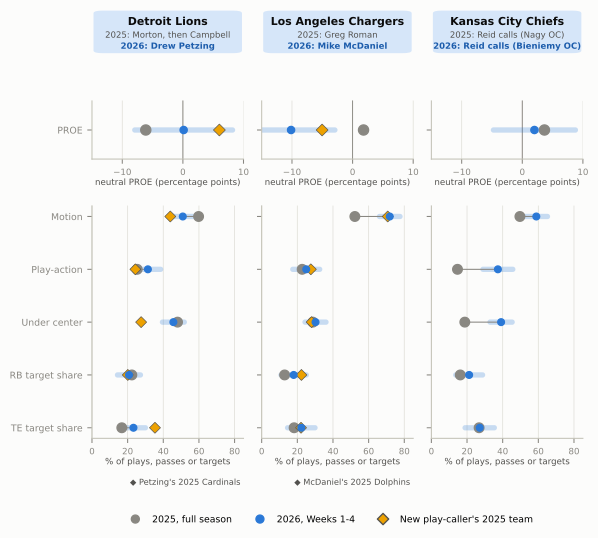
Figure 73.9: Coordinator-change usage cards: 2025 (grey) against 2026 Weeks 1-4 (blue, with a bar showing about ±2 standard errors of sampling noise), and the new play-caller’s previous team in 2025 (gold diamond) where there is one. Where a grey ring shows around a blue dot, nothing moved (Kansas City’s tight-end share). Top row: neutral-situation PROE, in percentage points. Bottom row: how the offense plays, as percentages: motion (any motion before or at the snap, FTN definition), play-action (share of passes), under center (share of plays), and the share of targets that went to running backs and to tight ends. Read across a card: where the blue dot has moved toward the gold diamond, the new play-caller’s habit has arrived; a move smaller than the bar is not yet evidence. Data: nflverse play-by-play and FTN charting; regular seasons.

Read the three cards one at a time, the way you would read a scouting report.

Los Angeles: the fingerprint arrived on day one. The Chargers used motion on 52% of their plays in 2025 under Roman. Through four games under McDaniel, the rate is 72%, almost exactly what his last Miami offense did (71%), and the jump is far outside the noise bar. The offense has also leaned hard on the run: a neutral PROE of about −10 after +2 in 2025. McDaniel’s habit and Harbaugh’s identity point the same way here (McDaniel’s 2025 Dolphins were about −5), so don’t credit the coordinator alone, and the PROE is noisier than the motion rate.

The fantasy lesson is in the targets, and it runs against McDaniel’s fingerprint. His Miami offenses concentrated the ball on two receivers. Through four weeks in Los Angeles no Charger has drawn even 18% of the targets: second-year receiver Tre Harris leads at about 18%, while Ladd McConkey, who drew about 21% in the 2025 games he played, is down to about 15%, the clearest loser so far. The backs’ share of the targets rose too. When a play-caller who funnels targets spreads them, the likeliest reason is the roster (he hasn’t found his Hill yet), not a new philosophy. The likelier bet is that the shares consolidate on whichever receiver he can feature with motion and manufactured touches, but four weeks can’t say which; and in a run-first offense even the winner’s volume is capped. The clearer beneficiary is the lead back, Omarion Hampton, who took 52% of the Chargers’ runs.

Detroit: a fingerprint plus a roster move. The Lions’ tight end target share went from 17% to 23%, toward Petzing’s Arizona level, and Sam LaPorta drew about 20% of the targets. Play-action rose from 25% to 31%, and motion fell from 60% to 51%, toward the 44% of Petzing’s last Cardinals offense. Each move is about the size of the noise bar, so they are hints rather than proof. And not everything moved his way: Detroit is still under center on about 46% of its plays (48% in 2025), nowhere near Arizona’s 28%. Petzing has kept that piece of the offense he inherited, which is a reminder that a play-caller adapts to his line and his quarterback too.

Be honest about the tight end number as well. Arizona’s third of the targets was partly scheme and partly that Trey McBride was simply the Cardinals’ best receiver for three years; the scheme part travels to Detroit, the McBride part doesn’t. And LaPorta drew about 19% of the targets in the nine 2025 games he played, so much of the team’s rise is just a healthy LaPorta, not a new philosophy. (The 2025 “before” dots also mix two play-callers, Morton and then Campbell.) Who gives up the targets? So far, slightly, both receivers: Amon-Ra St. Brown from 31% to 29% and Jameson Williams from 19% to 16%, moves inside the noise for now, but the direction the fingerprint predicts.

The PROE jump (−6 to about 0) is harder to read. It isn’t the score: the Lions trailed on an average snap by about four points, but PROE is measured only in neutral situations, where they were roughly level, and xpass already allows for the score. It is about one and a half noise bars, so it is a lean, pointing toward Petzing’s pass-first Arizona (+6), not proof. The clearest change is not scheme at all: with Montgomery traded, Gibbs took 83% of Detroit’s runs, up from 56%. That is a usage change you could have predicted in March.

Kansas City: same play-caller, different ingredients. Reid still calls the plays, so the theory says little should change, and the PROE barely did. But the Chiefs have been under center on 39% of plays (19% in 2025) and have used play-action on 37% of passes (15% in 2025), both far outside the noise. That pattern fits a team built around a new lead back, Walker, who took 76% of the Chiefs’ runs (and about 16% of the targets). It may also be Bieniemy: a coordinator who doesn’t call plays still builds the weekly game plan, the run-game install and the situational packages, and four games can’t separate his influence from Walker’s. Either way the lesson is the first step of the method: when the play-caller hasn’t changed, look for the roster change and the game plan, not a new fingerprint.

CautionCommon misconception

“Four weeks in, the new offense is clearly X.” Four games are about 240-260 plays and 120-180 neutral-situation plays per team. With that many plays, a team’s PROE has a standard error of about 4 percentage points, so a change of 5 or 6 points can be noise. Rates measured on every play (motion, under center) settle faster than rates measured on a subset (PROE, target shares). Big, consistent moves toward the new play-caller’s old numbers (the Chargers’ motion rate) are believable early; small moves, or moves against the fingerprint, need another month.

The same goes for a player’s own shares. In 2025, a receiver’s or tight end’s target share over Weeks 1-4 correlated about 0.67 with his share over the rest of the season, and the typical miss was about 5 percentage points: enough to tell a 30% alpha from a 15% third option, not enough to tell 22% from 26%.²⁰

Watch for it on Sunday

TipWatch for it on Sunday: the scheme-shift draft

Before the season (or now, for the 2026 test cases), pick one team with a new play-caller and write down a prediction for each skill position. Then check it after four weeks and again at mid-season.

Before kickoff (the forecast):

• Who calls the plays? If it’s the same person as last year, look for roster changes instead.
• His last offense’s fingerprint: neutral PROE, plays per game, motion and play-action rates, and the share of targets to RBs, TEs and WRs. Which way does each differ from this team’s last season?
• Translate it: which position’s share should rise, which should fall, and does the team’s total volume rise or fall? Name the player who gains most and the one who loses most.

During the game (the live check):

• Who’s on the field on third down and in the two-minute drill? That’s the passing-down back and the receivers the play-caller trusts.
• Does the tight end release or stay in? Count it for one quarter: on how many dropbacks did he run a route?
• Who’s in at the goal line? Watch the substitution inside the 5. That player owns the touchdowns.
• What’s the score? Discount the usage from a blowout: the leading team’s carries and the trailing team’s targets are game script, not role.

Predict the play

TipPredict the play 1: first-and-goal at the 2

off = line5() + [O("QB", "QB", -1.9, 0, "Q"), O("FB", "FB", -4.4, 0, "F"), O("G", "RB", -6.8, 0, "G"),
                 O("Y", "TE", -0.7, 4.8, "Y"), O("U", "TE", -0.7, -4.8, "U"), O("X", "WR", -1.5, -10.5, "X")]
dfn = [D("E1", "DE", 0.8, -6.2, "E"), D("T1", "DT", 0.8, -2.4, "T"), D("N", "DT", 0.8, -0.8, "T"),
       D("T2", "DT", 0.8, 0.8, "T"), D("T3", "DT", 0.8, 2.4, "T"), D("E2", "DE", 0.8, 6.2, "E"),
       D("L1", "MIKE", 2.8, -2.2, "M"), D("L2", "MIKE", 2.8, 2.2, "M"), D("L3", "SAM", 1.4, 7.8, "S"),
       D("C1", "CB", 1.2, -10.5, "C"), D("S1", "SS", 3.6, 0.0, "SS")]
pg = Play(off, dfn, los=108, to_go=2)
pg.highlight("Y", "U", "FB", color=TE_RING)
pg.highlight("G", color=WATCH)
fld = pg.draw(lateral=(-14.5, 14.5), window=(-9.5, 6.0), title=False)
no_numbers(fld.ax)
say(fld, pg, "goal line", (2.9, 10.6), fs=6.5, color=style.INK_2)
say(fld, pg, "lead back: on the sideline\nG, the backup, came in", (-6.0, 8.0), fs=6.3, color=style.INK_2)
plt.show()

Figure 73.10: First-and-goal at the 2, third quarter, score tied (illustrative). The offense is in 22 personnel from the I-formation: two tight ends attached to the line (Y and U, gold rings), the quarterback under center, a fullback (F, gold ring) and a tailback, G (green ring), stacked behind him, and one receiver, X. The team’s lead back, who has played most of the snaps today, jogged off as this group came on; G is the backup. The defense has answered with its goal-line package, nearly all of it within four yards of the line.

Who is the likely ball carrier? And what does this substitution tell a fantasy manager who owns the lead back, or is thinking of picking up G?

TipAnswer

A run, most likely to G behind the fullback. Two tight ends attached, a fullback, the quarterback under center and one receiver add up to a run-first goal-line call: a lead play or power with F leading through the hole. Play-action to a tight end is the main alternative, which is why goal-line defenses still keep a safety and a corner on their heels. A quarterback sneak is possible, but at the 2 rather than the 1 it is a less natural call for most teams.

The usage lesson is the substitution, not the play. The coaches took their lead back off the field at the 2. If they do it every time they get close, G owns the goal-line role, and the touchdowns go with it: the Seattle pattern from earlier in the chapter, where the back with fewer carries scored more than twice as many rushing touchdowns. For the lead back’s manager it caps his touchdown total, however many yards he gains between the 20s. For G, it is the opening’s “14 snaps, two touchdowns” backup, and the question to answer before picking him up is whether this happens every week. Watch the next few trips inside the 5. If it is G every time, he is a touchdown-dependent but real option in standard scoring, and less of one in PPR unless he also catches passes. Had this been the 1-yard line for a team with a tush-push quarterback, the answer would change again: the quarterback takes the ball, as Philadelphia’s did in the film room.

TipPredict the play 2: the receiver who changes teams

A wide receiver drew 25% of his old team’s targets as its clear number one. That team ran 64 plays a game and dropped back to pass on 62% of them. He signs with a team whose new play-caller’s last offense ran 58 plays a game and dropped back on 54%. On both teams about 87% of dropbacks end in a target (the rest are sacks, scrambles and throwaways). The new play-caller’s offenses have also thrown about 30% of their targets to tight ends, against 18% on the receiver’s old team, and the new team has a good tight end.

Use the volume equation: roughly how many targets per game should you forecast for him, before and after the move? What in the new offense could cut his share, and what would make you raise the forecast during the season?

TipAnswer

About 7 a game, down from about 8.6. Work the equation one term at a time. Old team: 64 plays × 0.62 pass rate × 0.87 target rate ≈ 34.5 team targets a game, and 25% of that is about 8.6. New team: 58 × 0.54 × 0.87 ≈ 27.2 team targets, and 25% of that is about 6.8. Same player, same share, about a fifth fewer targets: roughly 30 over a 17-game season, and at a typical two-thirds catch rate about 20 fewer catches (20 PPR points) before you count a single lost yard.

The share is the term to argue about. His 25% is his role as a clear number one, and that part tends to travel. But the new play-caller’s position split sends about 30% of the targets to tight ends instead of 18%. Those 12 extra points of share come from somewhere, usually the second and third receivers first, but a number one can lose a couple of points too. A forecast of 22-25% (6-7 targets a game) is the honest range.

Raise it if, after a month, his share is clearly above that range (28-30%, beyond the typical 5-point early miss), meaning the play-caller is building around him more than his history suggests; if the team throws more than its play-caller’s history (a higher PROE, or more snaps from a faster pace); or if the tight end gets hurt. Be careful with extra passing that comes from trailing: that is game script, not taste, and it won’t hold in the weeks the team keeps it close.

TipPredict the play 3: third-and-8, down 10 in the fourth

off = line5() + [O("QB", "QB", -5.0, 0, "Q"), O("RB", "RB", -5.2, -2.1, "B"),
                 O("X", "WR", -0.7, -15.0, "X"), O("Y", "TE", -1.5, 8.0, "Y"),
                 O("H", "WR", -1.5, 11.5, "H"), O("Z", "WR", -0.7, 17.0, "Z")]
dfn = [D("E1", "DE", 1.0, -5.5, "E"), D("T1", "DT", 1.0, -1.2, "T"), D("T2", "DT", 1.0, 2.0, "T"),
       D("E2", "DE", 1.0, 5.8, "E"), D("M", "MIKE", 5.0, 0.8, "M"), D("D1", "NB", 6.0, 11.5, "$"),
       D("D2", "DB", 6.0, 7.5, "D"), D("LCB", "CB", 7.0, -15.0, "C"), D("RCB", "CB", 7.5, 17.0, "C"),
       D("FS", "FS", 13.0, -6.0, "FS"), D("SS", "SS", 13.0, 9.0, "SS")]
pt = Play(off, dfn, los=45, to_go=8)
pt.highlight("RB", color=WATCH)
pt.highlight("Y", color=TE_RING)
fld = pt.draw(lateral=(-19, 21), window=(-7, 14.6), title=False)
no_numbers(fld.ax)
plt.show()

Figure 73.11: Third-and-8, fourth quarter, the offense trailing by 10. 11 personnel in trips: three receivers to the right (Z wide, H and the tight end Y, gold ring, detached into the slots) and X alone on the left, the quarterback in the shotgun and a running back (B, green ring) beside him. This team has two backs: A, its early-down runner, who had 18 carries and 1 catch in the first three quarters, and B. The defense is in dime: six defensive backs ($ the nickel, D the sixth), two safeties deep and only five men in the box.

Run or pass? Who on the offense is likely to touch the ball, and what kind of fantasy player is B?

TipAnswer

A pass, very likely, and B is the passing-down back. The situation alone makes it a pass: third-and-8 is a passing down at any score, and in 2025 teams trailing by 9 to 15 points in the fourth quarter threw on about four plays in five even before you add the down and distance. The personnel agree: three receivers to one side, the quarterback in the gun, and the defense in dime, expecting a throw.

The back on the field tells you about usage. The team swapped its early-down runner, A, for B, a back it trusts to pick up a blitzer and run a route, which is why B is on the field when the team must throw. Expect B to stay in to block if the defense shows pressure, and to release to the flat or over the middle as a checkdown if it doesn’t. The slot receivers, H and the detached tight end Y, are the other likely targets on a throw aimed just past the line to gain. And if the offense does run, it will be a draw to B: with only five defenders in the box, a draw against dime is the one run coordinators like on third-and-long, and it’s another reason B rather than A is out there.

For fantasy, B is the classic PPR back: few carries, but targets in exactly the game scripts where his team trails. In standard scoring he is barely worth a roster spot; in PPR, on a team that trails often, he can be a weekly starter, the 2025 Kenny Gainwell profile. A, meanwhile, is a game-script player: valuable when his team leads, invisible when it doesn’t.

Takeaways

• Fantasy points are outputs; usage is the input the scheme controls. Opportunity statistics (target share, air-yards share, WOPR, route participation) repeat from season to season far better than efficiency, and touchdowns barely repeat at all.
• Read receivers in order: on the field, running a route, targeted, targeted deep, productive per route. Snap share hides blocking snaps; route participation and YPRR fix that, and a productive part-timer whose role grows is the cheapest upside in fantasy.
• A running back’s touchdowns belong to whoever has the goal-line job. Snap share and carries describe the role between the 20s; red-zone share, and especially who gets the ball inside the 5 and the 2, decides the scoring. In 12 personnel the tight end is a receiver only if he runs routes.
• Volume = plays × pass rate × target rate × share. PROE sets the team’s taste and moves volume, not a number one’s share; pace adds or subtracts plays for everyone; game script overrides both late in games, and the betting lines forecast it (a big favorite’s extra plays are runs and touchdowns).
• Know the format and the price. PPR rewards catches and lifts pass-catching backs and slot receivers. ADP is a market price set by points above replacement, which is why fantasy running backs are dear when NFL ones are cheap; value is beating that price, most often by spotting a usage change the box score hasn’t shown.
• When the play-caller changes, his fingerprint travels; his old stars don’t. Check who calls plays and what the head coach wants, what his last offense did and how much of it was its players, and what roster he inherited; name a loser as well as a winner; then verify with a month of data, trusting every-play rates sooner than shares.

Connections

Builds on: Building a Roster (positional value, surplus value and scheme fit, the real-football versions of this chapter’s market); Tendencies: PROE, Personnel, Motion, and Coverage (where PROE and the neutral-situation filter come from, and how to measure a team’s motion and play-action habits); Working with nflverse Data in Python (the play-by-play, participation and FTN data behind every chart here); Personnel Groupings and Formation Rules and Vocabulary (the tight end’s two alignments); Pass Protection (why backs and tight ends stay in); and Red Zone, Goal Line, and Short Yardage (the tush push and the goal-line packages that decide touchdown shares).

Sets up: the Capstone, whose live checklist uses the same on-field reads (who’s in on third down, who’s in at the goal line, does the tight end release) as part of a full pre-snap routine. The case studies show the fingerprints this chapter measures in their original homes: the Shanahan tree (McDaniel’s motion and wide zone), the Chiefs (Reid’s play-calling across three coordinators) and the Lions (the offense Petzing inherits).

NoteGo deeper

Josh Hermsmeyer’s air-yards work (archived at FiveThirtyEight and in his later writing) is the foundation of WOPR, RACR (receiver air conversion ratio: receiving yards per air yard thrown his way) and the habit of reading opportunity before production. The nflverse data dictionary documents the target_share, air_yards_share and wopr columns that load_player_stats() computes for every player and week, and nflverse’s load_ff_opportunity() adds expected fantasy points built from usage (each carry and target valued by where it happened), which is this chapter’s idea turned into a model. For route-level data, PFF and FTN chart routes run by every player; snap counts are free through load_snap_counts(), and betting lines for every game sit in nflverse’s schedules (spread_line, total_line). To extend the chapter’s charts, change the season in the data cell, or swap the neutral() filter for your own definition and watch how the PROE ranking moves.

---

1. Default ESPN settings (10 teams, 16 rounds, PPR; one QB, two RB, two WR, one TE, one RB/WR/TE flex, one D/ST, one K and seven bench spots): 4for4, “An Expert’s Cheat Sheet to Dominating ESPN Fantasy Football Drafts” (2025): https://www.4for4.com/2025/preseason/experts-cheat-sheet-dominating-espn-fantasy-football-drafts . Commissioners can change every one of these settings.

2. Course calculation from nflverse regular-season play-by-play (2024-2025) and load_participation() (FTN-sourced for both seasons): wide receivers and tight ends with 50 or more targets in both seasons (n = 78); for a player with two teams in a season, the team where he drew more targets. Target share and air-yards share are measured against the team’s totals in the games the player was on the field; two-point tries excluded. “Route participation (est.)” is the share of the team’s dropbacks (qb_dropback == 1, which includes sacks and scrambles) on which the player was listed on the field, and “yards per route run (est.)” divides receiving yards by those dropbacks; true route counts come from PFF or FTN film charting and are lower for anyone who sometimes blocks.

3. Course calculation from nflverse load_player_stats() (regular season): Hill drew 30.2% of Miami’s targets in 2022 and 31.1% in 2023; Waddle 20.8% and 18.9%. McDaniel was Miami’s head coach and play-caller in both seasons (see the Shanahan tree case study).

4. The formula as implemented in nflverse: “wopr: Weighted Opportunity Rating, 1.5 × target_share + 0.7 × air_yards_share,” nflreadr data dictionary, player stats: https://nflreadr.nflverse.com/articles/dictionary_player_stats.html . Hermsmeyer as its creator, alongside RACR and PACR: Action Network, “WOPR” explainer: https://www.actionnetwork.com/article/p/601206703 ; Dynasty Nerds, https://www.dynastynerds.com/?p=33320 ; 4for4 author page (“creator of airyards.com and Air Yards based metrics PACR, RACR and WOPR”): https://www.4for4.com/users/josh-hermsmeyer/author-page . Hermsmeyer’s original airyards.com write-up is no longer online; the weights here are the ones every secondary source and nflverse use.

5. Course calculation on the same 78 receivers and tight ends as the stability chart: correlation of 2024 WOPR with 2025 PPR points per game 0.58, of 2024 target share 0.57, of 2024 air-yards share 0.48. Within a season (2025, 106 receivers and tight ends with 50+ targets), target share tracked PPR points per game more closely than WOPR did (0.84 against 0.76). Small samples; treat the two as roughly equal.

6. Course calculation from nflverse 2025 participation data (FTN-sourced personnel): the Rams were in 13 personnel on 21% of their dropbacks, and Nacua was on the field for 42% of those and 85% of their 11-personnel dropbacks; his share of the dropbacks was 59% in Week 6 and zero in Week 7.

7. FanDuel Research, “Fantasy Football: It’s Never Been Easier to Draft Saquon Barkley” (July 2024): https://www.fanduel.com/research/fantasy-football-it-s-never-been-easier-to-draft-saquon-barkley (FantasyPros consensus half-PPR ADP, pick 17 and RB6, “his lowest ADP in seven seasons,” i.e. of his career; the article uses July 2024 ADP data). ADP kept moving in August, so treat 17 as the July price.

8. Course calculation from nflverse 2024 regular-season play-by-play and load_player_stats(): 345 carries, 2,005 yards, 13 rushing touchdowns in 16 games; 33 catches on 43 targets for 278 yards and 2 touchdowns; 58% of the Eagles’ runs (scrambles included); 322.3 standard and 355.3 PPR fantasy points (first and second among running backs). Eagles’ neutral PROE −8.8, third-lowest. Snap share: Pro Football Reference snap counts via nflverse, 73% average. Inside the 2-yard line: Hurts 18 carries or targets and 11 touchdowns, Barkley 6 and 2. Pro Football Reference: https://www.pro-football-reference.com/players/B/BarkSa00.htm . Week 18: Nick Sirianni announced that Barkley and other starters would sit against the Giants with Philadelphia locked into the No. 2 seed (Detroit and Minnesota were playing for No. 1), leaving him 100 yards short of Eric Dickerson’s record: NBC Sports Philadelphia, https://www.nbcsportsphiladelphia.com/nfl/philadelphia-eagles/eagles-inactives-saquon-barkley-officially-inactive-nfl-week-18/640273 ; SI, https://www.si.com/nfl/eagles/onsi/news/eagles-saquon-barkley-gets-honest-about-sitting-week-18-pat3 .

9. Course calculation from nflverse load_player_stats(), 2024 regular season: Hurts 2,903 passing yards, 18 passing and 14 rushing touchdowns in 15 games, 315.1 standard fantasy points, eighth among quarterbacks. Pro Football Reference: https://www.pro-football-reference.com/players/H/HurtJa00.htm .

10. 12 personnel share: course calculation from nflverse participation data, regular-season pass and run plays (see Personnel Groupings). Fewer than three wide receivers: NFL Next Gen Stats via NFL.com, “NFL trend watch: Heavy personnel could shape Super Bowl LX showdown between Patriots and Seahawks”: https://www.nfl.com/news/nfl-trend-watch-heavy-personnel-could-shape-super-bowl-lx-showdown-between-patriots-and-seahawks .

11. Course calculation from nflverse 2025 participation and play-by-play, with this chapter’s on-field estimate (share of team dropbacks on the field, in games played): McBride 94%, LaPorta 92% (in his nine games), Higbee 59%, Parkinson 56%.

12. Course calculation from nflverse schedules (spread_line, total_line, the closing lines nflverse records) joined to 2025 regular-season play-by-play, by team-game: favorites by 7 or more (83 team-games) had an average score differential of +4.2 per snap, 26.3 runs and 34.6 dropbacks a game, and scored 28.2 points (implied 27.2); underdogs by 7 or more (91) had −7.8, 22.7 runs, 35.5 dropbacks and 16.9 points (implied 17.5). Kneels excluded. The spread’s correlation with the final margin, 2024-2025: 0.50.

13. “Fantasy football (gridiron),” Wikipedia: https://en.wikipedia.org/wiki/Fantasy_football_(gridiron) , on Wilfred “Bill” Winkenbach and the GOPPPL, whose rules were worked out in 1962 at a New York hotel during a Raiders road trip, with a first draft in August 1963; NFL.com, “Let’s play GOPPL: Digging out the roots of fantasy football”: https://www.nfl.com/news/let-s-play-goppl-digging-out-the-roots-of-fantasy-football-09000d5d80874333 . The original scoring paid only for touchdowns (rushing, receiving or passing), field goals, extra points and return touchdowns; yardage came later.

14. RotoWire, “What is PPR in fantasy football?”: https://www.rotowire.com/football/article/what-is-ppr-in-fantasy-football-94969 ; Sports Illustrated, “Fantasy Football 101: What Are PPR (Point Per Reception) Leagues?”: https://www.si.com/fantasy/fantasy-football-101-what-are-ppr-point-per-reception-leagues-01k0y4hz2k7n . The 2000s spread: the high-stakes NFFC adopted PPR at its founding in 2004 (founder Greg Ambrosius, NFFC forums: https://nffcforums.shgn.com/viewtopic.php?p=46813 ), and Footballguys added PPR scoring and rankings in 2008 (https://www.footballguys.com/article/Pasquino_Points_Per_Deception_2014 ). Site defaults: “ESPN’s default is full-point PPR, Yahoo’s is .5 PPR,” RotoWire: https://www.rotowire.com/football/article/weekly-rankings-41764 .

15. Footballguys, “Value-Based Drafting: The One Strategy Behind Every Strategy” (2026): https://www.footballguys.com/article/2026-value-based-drafting-one-strategy-behind-every-strategy ; Fantasy Sports & Gaming Association, “Joe Bryant elected to Fantasy Sports Hall of Fame”: https://thefsga.org/joe-bryant-elected-to-fantasy-sports-hall-of-fame . Sources date his first VBD articles to 1995-1996, and Bryant credited rotisserie-baseball writers for the underlying idea. The replacement-level chart is this book’s calculation from nflverse load_player_stats().

16. NFL.com, “Lions hiring former Cardinals offensive coordinator Drew Petzing as their new OC”: https://amp.nfl.com/news/lions-hiring-former-cardinals-offensive-coordinator-drew-petzing-as-their-new-oc ; CBS Sports, “Lions play-caller Drew Petzing fantasy football outlook 2026”: https://fantasy-api.cbssports.com/fantasy/football/news/lions-play-caller-drew-petzing-fantasy-football-outlook-2026/ . Staff history: this book’s fact sheet (Morton fired after 2025; Campbell called plays for the second half of 2025). Arizona’s tight-end target shares (33% in 2023, 34% in 2024, 35% in 2025): course calculation from nflverse play-by-play. The play-calling role was reported as part of the hire (ESPN, https://www.espn.com/nfl/story/_/id/47662766/sources-lions-finalizing-deal-hire-drew-petzing-new-oc ), and September 2026 coverage discusses “Petzing’s play-calling” (Fantasy Nerds, Sep. 15, 2026: https://www.fantasynerds.com/news/story/2026/09/15/detroit-lions-rushing-attack-surprises-in-week-1-victory-over-saints-1623808 ); no in-season report says Campbell has taken the calls back, but none states the arrangement outright either. Petzing’s background: Vikings offensive assistant and position coach 2014-2019 under Stefanski’s offensive staffs, then Browns tight ends coach from 2020 (Cleveland Browns, “Drew Petzing named Browns tight ends coach”: https://www.clevelandbrowns.com/news/drew-petzing-named-browns-tight-ends-coach ) and quarterbacks coach in 2022 (Cleveland Browns, “Browns announce additions, changes to 2022 coaching staff”: https://www.clevelandbrowns.com/news/browns-announce-additions-changes-to-2022-coaching-staff ).

17. AP via News4JAX, “Lions trade Montgomery to Texans for Scruggs, 4th, 7th-round picks, AP source says” (Mar. 2, 2026): https://www.news4jax.com/sports/2026/03/02/lions-trade-montgomery-to-texans-for-scruggs-4th-7th-round-picks-ap-source-says/ . NFL Network reported different compensation; the trade itself is confirmed by nflverse 2026 rosters.

18. Chargers.com, “Mike McDaniel, Chris O’Leary named new coordinators” (2026): https://www.chargers.com/news/mike-mcdaniel-chris-oleary-new-coordinator-2026 ; AP via News4JAX, “Mike McDaniel joins Harbaugh, Herbert as Chargers’ offensive coordinator after Dolphins firing” (Jan. 26, 2026): https://www.news4jax.com/sports/2026/01/26/mike-mcdaniel-joins-harbaugh-herbert-as-chargers-offensive-coordinator-after-dolphins-firing/ . Miami’s motion rates (FTN is_motion, motion before or at the snap: 68% in 2022, 79% in 2023, 76% in 2024, 71% in 2025) are this book’s calculation from nflverse FTN charting. Roman, the Chargers’ OC and play-caller in 2024 and 2025, was fired on Jan. 13, 2026, two days after the wild-card loss to New England: CBS Sports, https://www.cbssports.com/nfl/news/chargers-fire-offensive-coordinator-greg-roman-five-candidates-to-maximize-justin-herbert/ .

19. Chiefs.com, “Chiefs name Eric Bieniemy as offensive coordinator” (Jan. 2026): https://www.chiefs.com/news/chiefs-name-eric-bieniemy-as-offensive-coordinator ; A to Z Sports, “Andy Reid confirms suspicions about whether new OC Eric Bieniemy will call Kansas City Chiefs’ plays in 2026”: https://atozsports.com/nfl/kansas-city-chiefs-news/chiefs-andy-reid-confirms-suspicions-about-whether-new-offensive-coordinator-eric-bieniemy-will-call-plays-in-2026/ (Jan. 26, 2026). Nagy’s 2017 stretch: NFL.com, “Andy Reid gives Chiefs play-calling role to Matt Nagy”: https://www.nfl.com/news/andy-reid-gives-chiefs-play-calling-role-to-matt-nagy-0ap3000000886304 . Walker: AP via KPTV, “Chiefs land Super Bowl MVP Kenneth Walker on a 3-year deal worth up to $45M, AP source says” (Mar. 9, 2026): https://www.kptv.com/2026/03/09/chiefs-land-super-bowl-mvp-kenneth-walker-3-year-deal-worth-up-45m-ap-source-says/ .

20. Course calculation from nflverse 2025 regular-season play-by-play: wide receivers and tight ends with at least 10% of their team’s targets after Week 4 (n = 92); team-level shares of targets in Weeks 1-4 against Weeks 5-18. Correlation 0.67; mean absolute difference 5.0 percentage points.