Constraint Theory: How Plays Talk to Each Other

Why the play that works best is the one an offense calls least, and how coaches build a game out of questions and answers

⬇ Printable PDF

import os
import re
import shutil
import numpy as np
import pandas as pd
import matplotlib.pyplot as plt
from matplotlib.colors import LinearSegmentedColormap
from matplotlib.patches import Circle, Ellipse, FancyArrowPatch, FancyBboxPatch, RegularPolygon
from gridiron import Play, Player, Field, technique, style, routes as r

PURPLE = style.SERIES[6]   # a ring colour that is neither offense blue nor defense orange
RED = style.SERIES[7]      # rings on the defender a play is built to punish
GREEN = "#0f7a55"          # darker aqua, for text and boxes on the light page


def O(key, pos, d, w, label=None):
    return Player(key, pos, "off", d, w, label=key if label is None else label)


def D(key, pos, d, w, label=None):
    return Player(key, pos, "def", d, w, label=label)


def line(labels=False):
    """Five offensive linemen; unlabeled except the center unless labels=True."""
    names = ["LT", "LG", "C", "RG", "RT"]
    return [O(k, k, -0.7, w, k if (labels or k == "C") else "")
            for k, w in zip(names, (-3.2, -1.6, 0.0, 1.6, 3.2))]


def offset_i(labels=False):
    """21 personnel, offset I, tight end right, receivers in reduced (tight) splits. Seven on the line:
    five linemen, Y and X; Z is off the ball, and Q, F and R are backs."""
    return line(labels) + [O("QB", "QB", -1.9, 0.0, "Q"), O("FB", "FB", -4.5, 1.5, "F"),
                           O("RB", "RB", -7.0, 0.0, "R"), O("Y", "TE", -0.7, 4.8, "Y"),
                           O("X", "WR", -0.7, -9.5, "X"), O("Z", "WR", -1.5, 9.5, "Z")]


def base_43():
    """A 4-3 over front with one deep safety (eight in the box) against the offset I."""
    return [D("WDE", "DE", 1.0, technique("5", -1), "E"), D("WDT", "DT", 1.0, technique("1", -1), "T"),
            D("SDT", "DT", 1.0, technique("3", 1), "T"), D("SDE", "DE", 1.0, technique("9", 1), "E"),
            D("SAM", "SAM", 4.0, 5.2, "S"), D("MIKE", "MIKE", 4.6, 1.0, "M"), D("WILL", "WILL", 4.6, -2.6, "W"),
            D("SS", "SS", 7.5, 7.0, "SS"), D("FS", "FS", 13.0, -0.5, "FS"),
            D("LCB", "CB", 6.5, -9.5, "CB"), D("RCB", "CB", 6.5, 9.5, "CB")]


def spread():
    """11 personnel, 2x2 shotgun in tight splits: X and Z on the line with the five linemen; H and Y off the ball."""
    return line() + [O("QB", "QB", -5.0, 0.0, "Q"), O("RB", "RB", -5.0, -2.0, "R"),
                     O("X", "WR", -0.7, -12.5, "X"), O("H", "WR", -1.5, -7.5, "H"),
                     O("Y", "TE", -1.5, 7.5, "Y"), O("Z", "WR", -0.7, 12.5, "Z")]


def mug_look():
    """Nickel pressure look: four linemen, both linebackers mugged in the A gaps, the nickel and strong safety
    walked up as edge threats (eight possible rushers), one deep safety."""
    return [D("LDE", "DE", 1.0, -4.6, "E"), D("LDT", "DT", 1.0, -2.6, "T"), D("RDT", "DT", 1.0, 2.6, "T"),
            D("RDE", "DE", 1.0, 4.6, "E"), D("MIKE", "MIKE", 2.2, 0.85, "M"), D("WILL", "WILL", 2.2, -0.85, "W"),
            D("NB", "NB", 3.0, -6.6, "$"), D("SS", "SS", 4.0, 6.6, "SS"), D("FS", "FS", 13.0, -1.0, "FS"),
            D("LCB", "CB", 7.0, -12.5, "CB"), D("RCB", "CB", 7.0, 12.5, "CB")]


def threat(fld, p, *keys):
    """Dashed brown rings: defenders threatening to blitz before the snap (not the play's target)."""
    for k in keys:
        x, y = _P(fld, p, p.players[k].d, p.players[k].w)
        fld.ax.add_patch(Circle((float(x), float(y)), 1.25, fc="none", ec=style.BALL, lw=1.5, ls=(0, (2.2, 1.4)),
                                zorder=7))


def go_to(p, key, end, kind="block", delay=0.0, speed=None, via=()):
    """Move `key` through absolute (d, w) points `via` to `end`, as a block, path, run, route or pull."""
    start = np.array(p._cur(key))
    pts = [tuple(np.array(q) - start) for q in (*via, end)]
    if kind == "block":
        return p.block(key, pts=pts, delay=delay, speed=speed)
    if kind == "pull":
        return p.pull(key, pts=pts, delay=delay, speed=speed)
    if kind == "route":
        return p.route(key, pts, frame="field", delay=delay, speed=speed)
    return {"path": p.path, "run": p.run}[kind](key, pts, delay=delay, speed=speed)


def oz_first_second(p, fake=False):
    """The shared first second of the outside-zone family: every lineman steps right, Q opens right
    (and on a fake the back runs the outside-zone track without the ball)."""
    for k in ("LT", "LG", "C", "RG", "RT"):
        p.block(k, pts=[(0.2, 1.4)])
    go_to(p, "QB", (-3.3, 1.7), "path", speed=3.0)
    if fake:
        go_to(p, "RB", (-1.2, 4.6), "path", via=[(-5.6, 1.6), (-2.6, 3.8)])


def _P(fld, p, d, w):
    return fld.xy(*p.to_abs(d, w))


def say(fld, p, d, w, text, color=style.INK_2, fontsize=7.0, ha="center", weight="normal"):
    """A short on-field label at (d, w)."""
    x, y = _P(fld, p, d, w)
    fld.ax.text(x, y, text, fontsize=fontsize, color=color, ha=ha, va="center", zorder=11, fontweight=weight,
                linespacing=1.1, bbox=dict(boxstyle="round,pad=0.18", fc=style.SURFACE, ec="none", alpha=0.92))


def point_to(fld, p, text_at, target, text, color=style.INK_2, fontsize=6.8):
    """A label with a thin leader line to the player or spot it names."""
    (xt, yt), (xp, yp) = _P(fld, p, *text_at), _P(fld, p, *target)
    fld.ax.annotate(text, (float(xp), float(yp)), xytext=(float(xt), float(yt)), fontsize=fontsize,
                    color=color, ha="center", va="center", zorder=11, linespacing=1.1,
                    arrowprops=dict(arrowstyle="-", color=color, lw=0.7, shrinkA=2, shrinkB=7),
                    bbox=dict(boxstyle="round,pad=0.18", fc=style.SURFACE, ec="none", alpha=0.92))


def badge(fld, p, d, w, text, color=RED, fontsize=7.0):
    """A small numbered disc that ties a defender to a box elsewhere in the figure."""
    x, y = _P(fld, p, d, w)
    fld.ax.text(x, y, text, fontsize=fontsize, color="white", ha="center", va="center", zorder=12,
                fontweight="bold", bbox=dict(boxstyle="circle,pad=0.18", fc=color, ec="white", lw=0.6))


def ghost(fld, p, pts, color=style.DEFENSE, lw=1.4, alpha=0.55, zorder=5):
    """A faint dashed arrow through absolute (d, w) points: what a player did on earlier snaps."""
    xs, ys = _P(fld, p, np.array([q[0] for q in pts]), np.array([q[1] for q in pts]))
    fld.ax.plot(xs[:-1], ys[:-1], color=color, lw=lw, ls=(0, (3, 2)), alpha=alpha, zorder=zorder)
    fld.ax.add_patch(FancyArrowPatch((xs[-2], ys[-2]), (xs[-1], ys[-1]), arrowstyle="-|>", mutation_scale=10,
                                     color=color, lw=lw, alpha=alpha, ls=(0, (3, 2)), zorder=zorder))


def was_here(fld, p, d, w, to=None):
    """A faint dashed outline where a defender started, and (optionally) a dashed arrow to where he is now."""
    x0, y0 = _P(fld, p, d, w)
    fld.ax.add_patch(RegularPolygon((float(x0), float(y0)), 4, radius=0.95, orientation=np.pi / 4, fc="none",
                                    ec=style.DEFENSE, lw=0.9, ls=(0, (2, 1.5)), alpha=0.8, zorder=6))
    if to is not None:
        ghost(fld, p, [(d, w), to], alpha=0.9, lw=1.5)


def shifted(defense, **spots):
    """The defense with some players drawn where they have moved to: shifted(base_43(), WILL=(4.6, 0.2))."""
    return [q.moved(d=spots[q.key][0], w=spots[q.key][1]) if q.key in spots else q for q in defense]


def clean(ax):
    """Zoomed diagrams: drop hash ticks and yard numbers, and clip text to the window."""
    for ln in list(ax.lines):
        xs, ys = ln.get_data()
        if len(xs) == 2 and ln.get_linewidth() == 0.5 and np.hypot(xs[1] - xs[0], ys[1] - ys[0]) < 1.0:
            ln.remove()
    for t in list(ax.texts):
        if t.get_text().isdigit() and t.get_alpha() == 0.55:
            t.remove()
        else:
            t.set_clip_on(True)


def draw(p, ax=None, width_in=5.8, **kw):
    fld = p.draw(ax=ax, width_in=width_in, title=False, **kw)
    clean(fld.ax)
    return fld


def panel_title(ax, text, fontsize=8.6):
    ax.set_title(text, fontsize=fontsize, loc="left", color=style.INK, fontweight="bold", pad=3)


def pdf_build():
    return os.environ.get("RTG_FORMAT", "").lower() in ("pdf", "typst", "print")


# ---- frame strips (print) and videos (web) for simulated plays
MARK_R = 0.6    # frame-strip marker radius in yards, smaller than the static diagrams'


def tracking(play):
    df = play.to_tracking()
    df["_id"] = df["displayName"].astype(str)
    return df


def panel(ax, play, df, t, lateral, window, rings=()):
    """One moment of a simulated play: markers, trails of on-screen players, rings."""
    tmap = df.groupby("frameId")["time"].first()
    fid = int((tmap - t).abs().idxmin())
    ylo, yhi = sorted((play.ball_y - lateral[0], play.ball_y - lateral[1]))
    fld = Field(ax=ax, orient="vertical", los=play.los, window=window, numbers=False, hashes=False,
                lateral=(ylo, yhi), to_go=play.to_go)
    cur = df[df["frameId"] == fid]
    shown = cur[cur["x"].between(play.los + window[0] + 0.4, play.los + window[1] - 0.4)
                & cur["y"].between(ylo + 0.4, yhi - 0.4)]
    ids = set(shown["_id"])
    trails = df[(df["frameId"] <= fid) & df["_id"].isin(ids) & (df["side"] != "ball")]
    for (_, side), g in trails.groupby(["_id", "side"]):
        xs, ys = fld.xy(g["x"].values, g["y"].values)
        ax.plot(xs, ys, color=style.OFFENSE if side == "off" else style.DEFENSE, lw=0.9, alpha=0.4, zorder=3)
    ppy = fld.pts_per_yard()
    for _, rr in shown.iterrows():
        x, y = (float(v) for v in fld.xy(rr["x"], rr["y"]))
        if rr["side"] == "ball":
            ax.add_patch(Ellipse((x, y + 0.45), 0.7, 0.42, fc=style.BALL, ec="white", lw=0.5, zorder=9))
            continue
        lab = str(rr.get("label", "") or "")
        if rr["side"] == "off":
            ax.add_patch(Circle((x, y), MARK_R, fc=style.OFFENSE, ec="white", lw=0.6, zorder=8))
            tc = "white"
        else:
            ax.add_patch(RegularPolygon((x, y), 4, radius=MARK_R * 1.3, orientation=np.pi / 4,
                                        fc=style.DEFENSE_TINT, ec=style.DEFENSE, lw=1.0, zorder=8))
            tc = style.INK
        fs = max(4.0, min(8.0, ppy * (0.8 if len(lab) <= 1 else 0.6)))
        ax.text(x, y, lab, ha="center", va="center", fontsize=fs, color=tc, fontweight="bold", zorder=10)
    for key, col in rings:
        rr = cur[cur["displayName"] == key].iloc[0]
        x, y = fld.xy(rr["x"], rr["y"])
        ax.add_patch(Circle((float(x), float(y)), 1.05, fc="none", ec=col, lw=1.7, zorder=7))
    return fld


def strip(play, times, notes, lateral, window, ncols=2, rings=(), width_in=6.4):
    """Numbered, captioned frame strip: the PDF stand-in for the video."""
    df = tracking(play)
    nrows = int(np.ceil(len(times) / ncols))
    pw = width_in / ncols
    span_w, span_d = lateral[1] - lateral[0], window[1] - window[0]
    fig, axes = plt.subplots(nrows, ncols, squeeze=False,
                             figsize=(width_in, nrows * (pw * span_d / span_w + 0.5)))
    for ax in axes.flat[len(times):]:
        ax.axis("off")
    for i, (ax, t) in enumerate(zip(axes.flat, times)):
        panel(ax, play, df, t, lateral, window, rings)
        ax.set_title(f"{i + 1}.  " + ("snap" if abs(t) < 1e-6 else f"{t:+.1f} s"), fontsize=8.5,
                     color=style.INK_2, loc="left")
        ax.text(0.5, -0.03, notes[i], transform=ax.transAxes, ha="center", va="top", fontsize=7.5,
                color=style.INK, linespacing=1.15)
    fig.tight_layout(h_pad=1.4, w_pad=0.6)
    return fig


def video(play, times, notes, lateral, window, rings=(), width_in=5.6):
    """Web version of the strip: every frame, with the strip's notes as running captions."""
    from matplotlib import animation
    from IPython.display import HTML, display
    df = tracking(play)
    span_w, span_d = lateral[1] - lateral[0], window[1] - window[0]
    fig, ax = plt.subplots(figsize=(width_in, width_in * span_d / span_w + 0.4))
    tmap = df.groupby("frameId")["time"].first()

    def update(fid):
        ax.clear()
        t = float(tmap[fid])
        panel(ax, play, df, t, lateral, window, rings)
        cur = [n.replace("\n", " ") for tt, n in zip(times, notes) if tt <= t + 1e-6]
        ax.set_title(("snap" if abs(t) < 0.05 else f"{t:+.1f} s") + (("   " + cur[-1]) if cur else ""),
                     fontsize=8.5, color=style.INK, loc="left")
        return []

    anim = animation.FuncAnimation(fig, update, frames=sorted(df["frameId"].unique()), interval=100)
    html = (anim.to_html5_video(embed_limit=40).replace("<video ", '<video style="max-width:100%;height:auto" ')
            if shutil.which("ffmpeg") else anim.to_jshtml(default_mode="once"))
    plt.close(fig)
    display(HTML(html))


def animation_or_strip(play, times, notes, lateral, window, rings=(), ncols=2):
    """Video on the website; a numbered, captioned frame strip in the PDF."""
    if pdf_build():
        strip(play, times, notes, lateral, window, ncols=ncols, rings=rings)
        plt.show()
    else:
        video(play, times, notes, lateral, window, rings=rings)

from gridiron.data import pbp, nfl

SEASONS = [2022, 2023, 2024, 2025]
PCOLS = ["season", "season_type", "game_id", "play_id", "posteam", "play_type", "down", "ydstogo", "wp",
         "half_seconds_remaining", "pass", "epa", "success", "drive", "yards_gained"]
GROUPS = ["11", "12", "13", "21", "22"]
ALIGN = {"U": "Under center", "S": "Shotgun", "P": "Pistol"}


def backs_tes(s):
    """'1 C, 2 G, 1 QB, 1 RB, 2 T, 1 TE, 3 WR' (or the pre-2023 '1 RB, 1 TE, 3 WR') -> '11'."""
    if not isinstance(s, str):
        return None
    n = {k: int(v) for v, k in re.findall(r"(\d+) ([A-Z]+)", s)}
    return f"{n.get('RB', 0) + n.get('FB', 0)}{n.get('TE', 0)}"


def n_linemen(s):
    """Offensive linemen on the field ('... 1 C, 2 G, 2 T ...' or a pre-2023 '6 OL'); 5 if not listed."""
    if not isinstance(s, str):
        return 5
    n = sum(int(v) for v, k in re.findall(r"(\d+) ([A-Z]+)", s) if k in ("C", "G", "T", "OL"))
    return n if n else 5


def neutral_plays(seasons):
    """Regular-season runs and dropbacks on first and second down, win probability 20-80%, outside the
    last two minutes of each half, with personnel (participation) and QB alignment (FTN charting)."""
    d = pbp(seasons, columns=PCOLS)
    d = d[(d["season_type"] == "REG") & d["play_type"].isin(["pass", "run"])].sort_values(["game_id", "play_id"])
    # was the previous snap of the same drive a run of 10+ yards? (for the "after the big run" check)
    prev = d.groupby(["game_id", "drive"])
    d["after_big_run"] = (prev["play_type"].shift(1) == "run") & (prev["yards_gained"].shift(1) >= 10)
    d["first_of_drive"] = prev["play_type"].shift(1).isna()
    d = d[d["down"].notna()]
    part = nfl().load_participation(seasons).to_pandas()[["nflverse_game_id", "play_id", "offense_personnel"]]
    ftn = nfl().load_ftn_charting(seasons).to_pandas()[["nflverse_game_id", "nflverse_play_id",
                                                        "qb_location", "is_play_action"]]
    d = d.merge(part, left_on=["game_id", "play_id"], right_on=["nflverse_game_id", "play_id"], how="left")
    d = d.merge(ftn, left_on=["game_id", "play_id"], right_on=["nflverse_game_id", "nflverse_play_id"],
                how="left")
    d["pers"] = d["offense_personnel"].map(backs_tes)
    d["ol"] = d["offense_personnel"].map(n_linemen)
    d = d[(d["down"] <= 2) & d["wp"].between(0.2, 0.8) & (d["half_seconds_remaining"] > 120)
          & d["qb_location"].isin(list(ALIGN)) & d["pers"].notna()].copy()
    d["align"] = d["qb_location"].map(ALIGN)
    d["group"] = d["pers"].where(d["pers"].isin(GROUPS), "other")
    d["look"] = d["group"] + " | " + d["align"]
    return d


def tendency_table(d, team=None, season=2024, groups=("11", "12", "13", "21")):
    """Pass rate and snap count by personnel group (rows) and quarterback alignment (columns)."""
    x = d[(d["season"] == season) & d["group"].isin(groups)]
    if team:
        x = x[x["posteam"] == team]
    cols = ["Under center", "Shotgun", "Pistol"]
    rate = x.pivot_table(index="group", columns="align", values="pass", aggfunc="mean")
    n = x.pivot_table(index="group", columns="align", values="pass", aggfunc="size")
    return (rate.reindex(index=list(groups), columns=cols),
            n.reindex(index=list(groups), columns=cols).fillna(0).astype(int))


def guess_from_film(d, min_other=8):
    """For every snap, what a scout would have predicted from the team's OTHER games that season:
    the pass rate of that personnel-and-alignment look (if seen at least `min_other` times elsewhere),
    and the team's overall pass rate. Leaving the game out keeps the guess honest."""
    out = d.copy()
    for name, keys in (("xp_look", ["season", "posteam", "look"]), ("xp_team", ["season", "posteam"])):
        g, gg = out.groupby(keys)["pass"], out.groupby(keys + ["game_id"])["pass"]
        n_other = g.transform("size") - gg.transform("size")
        p_other = (g.transform("sum") - gg.transform("sum")) / n_other.clip(lower=1)
        out[name] = p_other.where(n_other >= min_other)
    out["xp_look"] = out["xp_look"].fillna(out["xp_team"])
    out = out[out["xp_team"].notna()]
    out["hit_look"] = (out["xp_look"] > 0.5).astype(int) == out["pass"]
    out["hit_team"] = (out["xp_team"] > 0.5).astype(int) == out["pass"]
    out["said"] = np.select([out["xp_look"] < 0.45, out["xp_look"] > 0.55], ["run", "pass"], "toss-up")
    return out


N = neutral_plays(SEASONS)
G = guess_from_film(N)
ACC = G.groupby(["season", "posteam"])[["hit_look", "hit_team"]].mean()
ACC_SEASON = G.groupby("season")[["hit_look", "hit_team"]].mean()
R_DET, N_DET = tendency_table(N, "DET", 2024)
R_NFL, N_NFL = tendency_table(N, None, 2024)
RANK24 = ACC.loc[2024]["hit_look"].rank()
RANK25 = ACC.loc[2025]["hit_look"].rank()

# does breaking the tendency pay? EPA by what the look said and what the offense did
BRK = G[G["said"] != "toss-up"].groupby(["said", "pass"])["epa"].agg(["mean", "std", "size"])
BRK["se"] = BRK["std"] / np.sqrt(BRK["size"])
DB = G[(G["pass"] == 1) & (G["said"] != "toss-up") & G["is_play_action"].notna()].copy()
DB["pa"] = DB["is_play_action"].astype(bool)
PA_SPLIT = DB.groupby(["said", "pa"])["epa"].agg(["mean", "std", "size"])
PA_SPLIT["se"] = PA_SPLIT["std"] / np.sqrt(PA_SPLIT["size"])
PA_SHARE = DB.groupby("said")["pa"].mean()

phi = N[(N["season"] == 2024) & (N["posteam"] == "PHI") & (N["look"] == "11 | Pistol")]
PHI_N, PHI_PASS = len(phi), phi["pass"].mean()

# play-action on the snap right after a 10+ yard run (same drive), first-and-10 only so the down is the same
F10 = N[(N["down"] == 1) & (N["ydstogo"] == 10) & ~N["first_of_drive"] & (N["pass"] == 1)
        & N["is_play_action"].notna()].copy()
F10["pa"] = F10["is_play_action"].astype(bool)
AFTER_SHARE = F10.groupby("after_big_run")["pa"].mean()
AFTER = F10[F10["pa"]].groupby("after_big_run")["epa"].agg(["mean", "std", "size"])
AFTER["se"] = AFTER["std"] / np.sqrt(AFTER["size"])
AFTER_SEASONS = (F10[F10["pa"]].groupby(["season", "after_big_run"])["epa"].mean().unstack()
                 .pipe(lambda t: int((t[True] > t[False]).sum())))

# Detroit's sixth-lineman ("jumbo") snaps, 2022-2024
J = N[(N["ol"] >= 6) & N["season"].between(2022, 2024)]
DET_J = J[J["posteam"] == "DET"]
DET_J_N, DET_J_PASS = len(DET_J), DET_J["pass"].mean()
NFL_J_PASS = J["pass"].mean()
DET_J_PA = DET_J.loc[DET_J["pass"] == 1, "is_play_action"].astype(float).mean()

# is a hard-to-read offense a better one? team-season look accuracy vs EPA per play
TEAM_EPA = G.groupby(["season", "posteam"]).agg(hit=("hit_look", "mean"), epa=("epa", "mean"))
CORR = TEAM_EPA["hit"].corr(TEAM_EPA["epa"])


def pct(x, nd=0):
    return f"{100 * x:.{nd}f}%"

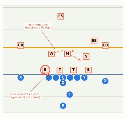
Second quarter, first-and-10 near midfield. For the fourth time today the offense comes out with two backs behind the quarterback and a tight end on the right, and for the fourth time every lineman takes the same step to his right at the snap. The first three times, the back ran behind that wall of blockers for 6, 4 and 9 yards, and by now the linebackers are flying to the right before the ball is even handed off. This time the quarterback fakes the handoff, turns his back to all of them and rolls left. The defensive end on that side has crashed down the line chasing the running back, and there is nobody within ten yards of the quarterback. His tight end is alone in the left flat. Twenty-two yards. “They set that up,” says the analyst. What does that actually mean? How does one play set up another, and if the bootleg is that good, why didn’t they call it on the first snap?

You’ll be able to:

• Tell a base play from a constraint play, name the defender each constraint play punishes, and explain why a constraint play’s average looks better than the base play’s even when it’s called the right amount.
• Recognize the illusion of complexity from both ends: the same play in different outfits, and different plays from the same look.
• Spot sequencing during a game: the counter after the flow, the play-action after the big run, the tendency breaker after a stretch of predictability.
• Explain what a self-scout looks for and what a team does with what it finds.
• Read the defense’s version: one pressure look, several coverages behind it.
• Build a team’s tendency table from nflverse data (personnel group by the quarterback’s alignment, the formation information the public data carries), and say how much the pre-snap look gave away.

NoteYou’ll need

• Perimeter Runs and Misdirection: series football (groups of plays that start alike and end differently, the Wing-T’s buck series), misdirection and eye candy, and the puzzle of the receiver run whose average beats a running back’s carry by a mile.
• Play-Action, Bootlegs, and Screens: play-action, the bootleg, the naked bootleg, the keeper and the shot play, and the finding that play-action does not need a successful run game, only a fake that looks exactly like the real run.
• What Beats What: the idea of a coverage beater, a pass concept built to beat a particular coverage, and why beaters are only probabilities. This chapter widens the same logic from one snap to a whole game.
• Helpful too: outside zone from Zone Running, the counter from Gap and Power Runs, and tells from How to Watch a Broadcast.

How to read the diagrams. Offense is blue circles, defense orange squares, and left and right are always the offense’s. Q is the quarterback, R the running back, F the fullback, Y the tight end, and X and Z the wide receivers; H is a slot receiver and U a second tight end. C is the center (the other linemen are labelled only where they matter). On defense, E and T are the ends and tackles, S, M and W the Sam, Mike and Will linebackers, $ the nickel back, CB the cornerbacks and FS and SS the safeties. Lines ending in a bar are blocks, arrows are paths, the thick dark arrow is the ball carrier, and a dashed brown arrow is the throw. A red ring marks the defender a play is built to punish, a purple ring a blocker or dropper to watch, and a green ring the ball carrier to follow. In the defense’s pictures a dashed brown ring marks a defender who is threatening to blitz before the snap.

Every play is an answer to a question

Start with what a defense is trying to do on every snap. It has eleven players and the offense has eleven, but the offense knows where the ball is going and the defense doesn’t. So the defense guesses, in an educated way. It studies the offense all week, learns what the offense likes, and on Sunday it leans. A linebacker who knows the offense runs outside zone half the time from this formation takes his first step toward the play side a little faster. A safety who has seen the tight end block on every snap creeps down to help against the run. A defensive end on the far side, told the cutback is where this offense hurts people, chases hard down the line.

Each of those leans makes the defense better against what the offense usually does. Each one also makes it worse against something else. The linebacker flying to the play side has left the middle of the field. The safety creeping down has nobody behind him. The end chasing down the line is no longer outside the quarterback. An offense that can see those leans, and that has a play aimed at each one, wins the argument.

That is the core of what coaches call constraint theory. Every offense has a small number of base plays: the handful of runs and passes it builds itself around, calls most often, and wants to be good at whatever the defense does. For a Shanahan-family offense the base play is outside zone; for a gap-scheme team it might be power; for a spread passing team it might be a quick-game concept or the inside-zone RPO. Then it has constraint plays: plays whose main job is to punish the defense for over-playing the base play. A constraint play works best exactly when the defense cheats against the base play, and its mere existence is what keeps the defense from cheating too much. The word comes from what it does to the defense: it constrains how far the defense can lean.¹

ImportantWhy it exists

A defense that knows what’s coming wins. Constraint plays exist so that the defense can never fully commit to stopping the base play: every lean has a price, and the offense collects it. The trade is that a constraint play is a specialist. It is usually a worse play than the base play when the defense hasn’t cheated (a bootleg into an end who stayed home is a sack waiting to happen, a counter into linebackers who didn’t flow runs straight into them), so it can’t become the offense’s main course. It lives on the base play’s reputation, and the base play lives on its protection. (If that sounds like it contradicts the receiver-run and play-action numbers from earlier chapters, where these plays win on average, hold the thought: the section “Why not just run the constraint play more?” below shows why their averages should look better anyway.)

The two kinds of play need each other. Without the constraint plays, the defense cheats freely and the base play dies. Without the base play, the constraint plays have nothing to punish: nobody chases a fake of a play that’s never run. This is why coaches talk about plays “talking to each other.” A good offense is not a list of good plays. It’s a set of plays in which each one’s weakness is another one’s strength.

You won’t often hear “constraint play” on a sideline or in a clinic talk. Coaches say the same thing in their own dialects: complementary plays, answers, if-then calls (“if the Will flows, then counter”), or the “play-pass off” a run. When a coordinator says a play “keeps them honest,” he is describing a constraint play.

NoteMadden vs. real life

In a video game you can find a play that works and call it until it stops working, and often it never does, because the computer’s defense doesn’t keep a scouting report on you. Real defenses do. They watch every snap you have run this season, they know what you like from every formation, and they adjust between series, at halftime and during the week. There is no best play in real football, only a best play given what the defense is doing about the others. That is also why the answer to “if the bootleg is so good, why not run it every time?” is the same as the answer to “why not throw deep every time?”: the defense would stop leaning, and the play would turn back into an ordinary one, or worse.

CautionCommon misconception

“Constraint plays are trick plays.” A few are (a flea-flicker, in which the back takes a handoff and pitches the ball back to the quarterback, who throws deep, is a constraint on safeties who come up to stop the run), but most are ordinary, bread-and-butter football: the bootleg, the screen, the draw, the counter, the quick throw behind a blitzing linebacker. What makes a play a constraint is not that it’s unusual. It’s that its job is defined by another play.

The constraint tree: outside zone and its family

The cleanest place to see constraint theory is the offense that has made it a way of life: the outside-zone system of Mike Shanahan’s Broncos in the 1990s (built with his offensive line coach Alex Gibbs, whose story is in Zone Running) and of his son Kyle’s 49ers today, and the many coaches who came out of it. Its base play is outside zone (wide zone), the run you met in that chapter: every lineman steps hard to one side, the back aims at the tight end’s outside leg, and the defense has to run sideways with the play or get outflanked. Outside zone trains a defense, snap after snap, to flow: to run hard to the play side. Every constraint play in the system is designed around a defender who has learned that lesson too well. How many plays is that? Fewer than a Madden menu suggests: a few base runs and a few base passes, each with a small family of answers like the one below. The exact count varies by staff, but the point of the system is that it is small enough to practice until every play looks the same for its first second.

fig = plt.figure(figsize=(6.6, 6.4))
cv = fig.add_axes([0, 0, 1, 1]); cv.set_xlim(0, 100); cv.set_ylim(0, 97); cv.axis("off")
axf = fig.add_axes([0.25, 0.555, 0.50, 0.425])
p = Play(offset_i(), base_43(), los=35, to_go=None)
for k in ("LT", "LG", "C", "RG", "RT"):
    p.block(k, pts=[(0.2, 1.4)])
go_to(p, "Y", (0.3, 5.8)); go_to(p, "FB", (3.0, 6.4), via=[(-2.6, 4.2)])
go_to(p, "QB", (-3.3, 1.7), "path", speed=3.0)
go_to(p, "RB", (5.0, 7.8), "run", via=[(-5.6, 1.6), (-2.6, 3.8), (0.0, 5.6)])
go_to(p, "MIKE", (4.0, 4.4), "path"); go_to(p, "WILL", (6.1, 2.6), "path", via=[(5.9, -0.6)])
go_to(p, "WDE", (0.0, -1.0), "path", via=[(0.5, -3.0)])
go_to(p, "SS", (4.6, 6.4), "path")
p.highlight("RB")
f = draw(p, ax=axf, lateral=(-11.5, 11.5), window=(-8.6, 10.5))
badge(f, p, 4.6, -0.8, "1"); say(f, p, 3.2, -0.8, "both LBs", fontsize=5.8, color=RED)
badge(f, p, 2.4, -5.4, "2"); badge(f, p, 6.1, -3.7, "3"); badge(f, p, 9.2, 7.0, "4")
axf.set_title("The base play: outside zone right", fontsize=9, loc="center", color=style.INK,
              fontweight="bold", pad=3)


def box(x, y, w, h, title, body, num):
    cv.add_patch(FancyBboxPatch((x - w / 2, y - h / 2), w, h, boxstyle="round,pad=0.4,rounding_size=1.4",
                                fc=style.SURFACE, ec=GREEN, lw=1.3, zorder=2))
    cv.text(x - w / 2 + 1.4, y + h / 2 - 1.4, title, ha="left", va="top", fontsize=8.2, fontweight="bold",
            color=style.INK, zorder=3)
    cv.text(x - w / 2 + 1.4, y + h / 2 - 5.6, body, ha="left", va="top", fontsize=6.8, color=style.INK_2,
            zorder=3, linespacing=1.2)
    if num:
        cv.text(x + w / 2 - 2.4, y + h / 2 - 2.4, num, fontsize=7, color="white", ha="center", va="center",
                fontweight="bold", zorder=4, bbox=dict(boxstyle="circle,pad=0.18", fc=RED, ec="white", lw=0.6))


def arrow(x0, y0, x1, y1):
    cv.add_patch(FancyArrowPatch((x0, y0), (x1, y1), arrowstyle="-|>", mutation_scale=11, color=style.DEFENSE,
                                 lw=1.3, zorder=1))


def why(x, y, text):
    cv.text(x, y, text, ha="center", va="center", fontsize=6.5, color=style.DEFENSE_DARK, style="italic",
            zorder=3, linespacing=1.15, bbox=dict(boxstyle="round,pad=0.2", fc=style.SURFACE, ec="none"))


W, H, YB = 22.5, 16, 33
xs = [12.5, 37.5, 62.5, 87.5]
box(xs[0], YB, W, H, "Bootleg", "fake right, roll left\nbehind a blocker (the\nprotected boot); crossers\nopen behind the flow", "1")
box(xs[1], YB, W, H, "Naked boot", "same fake; nobody\nblocks the end: he is\nbehind a quarterback\nrolling away", "2")
box(xs[2], YB, W, H, "Counter", "line and back start\nright; the ball comes\nback left behind a\npulling guard", "3")
box(xs[3], YB, W, H, "Play-action shot", "same fake, seven\nblock; throw deep\nbehind the safety\nwho came down", "4")
box(xs[1], 8.0, W, 12.5, "Keeper", "on the naked: nobody\nstayed outside, so\nthe quarterback runs", None)
top = 52.5
for x, txt in zip(xs, ["linebackers\nflow hard", "backside end\nchases the back", "backside linebacker\nover-runs the play",
                       "safety races\ndown to the run"]):
    arrow(50 + (x - 50) * 0.35, top, x, YB + H / 2 + 0.9)
    why(50 + (x - 50) * 0.70, top - 5.6, txt)
arrow(xs[1], YB - H / 2 - 0.6, xs[1], 8.0 + 6.25 + 0.9)
why(xs[1] + 14.5, 19.4, "the flat defender\nruns with the receivers")
cv.text(76, 8.5, "Every arrow is the defense cheating\nto stop the base play. If nobody\ncheats, the base play gets its yards,\nwhich is why the defense cheats.",
        ha="center", va="center", fontsize=7.2, color=style.INK, linespacing=1.25,
        bbox=dict(boxstyle="round,pad=0.5", fc=style.OFFENSE_TINT, ec="none"))
plt.show()

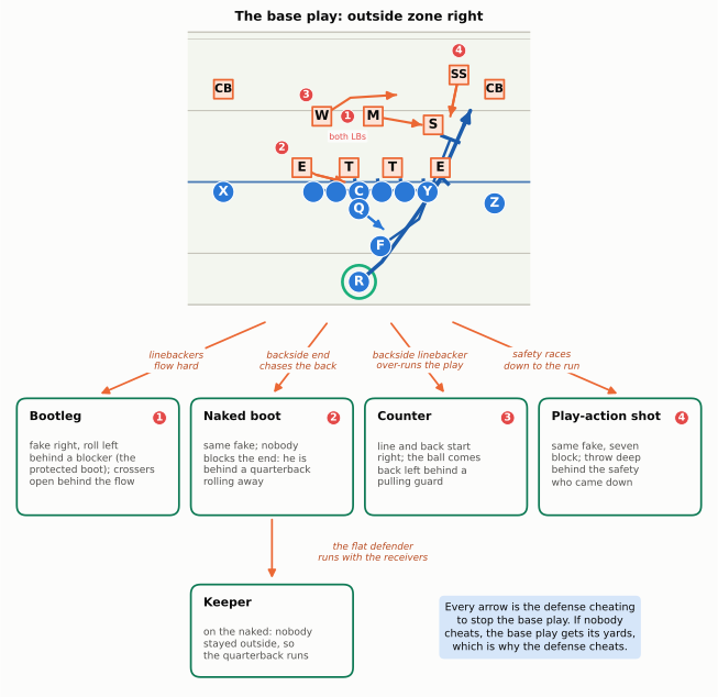
Figure 43.1: The constraint tree around outside zone (illustrative). Top: the base play, outside zone right, with four defenders numbered by how they learn to cheat against it. Below: the play that punishes each cheat. (1) Linebackers who flow hard with the line leave the middle behind them: the bootleg. (2) A backside end who chases the back down the line ends up behind a quarterback rolling away from him: the naked boot. (3) A backside linebacker who over-runs the play leaves the cutback side empty: the counter. (4) A safety who races down to help against the run leaves the deep middle open: the play-action shot. The keeper hangs off the naked boot: if the defender on that side runs with the receivers, nobody is left to stop the quarterback from running. The arrows also run backwards: if the defense cheats on none of them, outside zone gets its yards.

Read Figure 43.1 one branch at a time, starting from what the defense does wrong.

(1) Linebackers flow hard: the bootleg. Outside zone punishes slow linebackers; a linebacker who doesn’t beat his blocker to the play side gets sealed inside and the back runs past him. So linebackers learn to fly. The bootleg fakes outside zone one way and rolls the quarterback out the other way, behind a blocker (a pulling guard or the fullback) who takes care of the defensive end on that side; that blocker is why 04-05 also called it the protected boot. Receivers cross the field to meet him at three depths, and the crossing routes come open behind the linebackers who just ran the other way. The defense’s lesson (“flow fast”) is the very thing the bootleg cashes in.

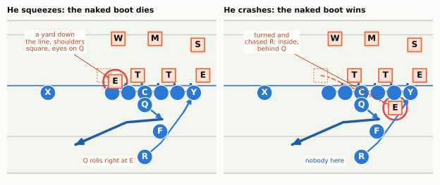
(2) The backside end chases: the naked boot. On outside zone, the defensive end on the far side (the backside) has two jobs that pull against each other. He is the man who stops the cutback: if he stays put, the back has a lane back to his side. But he is also the last defender on that edge, so his coaching, which you met in 03-05, is to squeeze while checking boot, counter, reverse: shuffle down the line a yard or two to shrink the cutback lane, keep his shoulders square and his eyes on the quarterback, and stay at the edge until he is sure the ball has gone the other way. That is the disciplined version, and it is hard to play. When the cutback has been hurting the defense, the end starts to crash instead: he turns his shoulders, flattens down the line and chases the back. Figure 43.2 shows the difference. Crashing is the cheat. The naked bootleg sends the quarterback right at the spot the crashing end just left, with no blocker for him (that’s the “naked”). The end who crashed is now behind a quarterback who is running away from him, and nobody else is close. If the end squeezed and stayed home instead, he is standing on the quarterback’s launch point, and the quarterback is in trouble, which is the price of a play that only works against a cheat.

fig, axes = plt.subplots(1, 2, figsize=(6.6, 3.5))
E0 = (1.0, technique("5", -1))                      # the end's alignment, a 5-technique
for ax, crash in zip(axes, (False, True)):
    e1 = (-2.2, 3.3) if crash else (0.4, -2.9)     # where he is when Q would start the boot
    dfn = shifted([q for q in base_43() if q.key not in ("LCB", "RCB", "SS", "FS")], WDE=e1)
    p = Play(offset_i(), dfn, los=35, to_go=None)
    oz_first_second(p, fake=True)
    go_to(p, "QB", (-5.8, -6.8), "run", via=[(-3.6, -1.8)], delay=0.1)
    p.highlight("WDE", color=RED)
    f = draw(p, ax=ax, lateral=(-13.0, 6.5), window=(-8.6, 6.4))
    # where he started: a faint outline and a dashed arrow to where he is now
    was_here(f, p, *E0)
    ghost(f, p, [E0, (E0[0] - 0.2, E0[1] + 0.9), e1] if crash else [E0, e1], alpha=0.9, lw=1.5)
    panel_title(ax, "He crashes: the naked boot wins" if crash else "He squeezes: the naked boot dies", fontsize=8.2)
    if crash:
        point_to(f, p, (4.3, -8.8), e1, "turned and\nchased R: inside,\nbehind Q", color=style.DEFENSE_DARK)
        say(f, p, -7.4, -3.6, "nobody here", fontsize=6.6, color=style.OFFENSE_DARK)
    else:
        point_to(f, p, (4.3, -8.8), e1, "a yard down\nthe line, shoulders\nsquare, eyes on Q", color=style.DEFENSE_DARK)
        say(f, p, -7.4, -3.6, "Q rolls right at E", fontsize=6.6, color=style.DEFENSE_DARK)
fig.tight_layout(w_pad=0.8)
plt.show()

Figure 43.2: Two ways to play the backside end (E, red ring) against outside zone right, at the moment the quarterback (Q) would start a naked boot to the left. Left, he squeezes: he shuffles a yard or two down the line with his shoulders square and his eyes on the quarterback (his checklist is boot, counter, reverse), so he is still at the edge, right on the spot the quarterback wants to roll to. Right, he crashes: he turns and chases the back flat down the line, which stops the cutback but leaves him inside and behind the quarterback. The naked boot beats the crash and dies against the squeeze.

The keeper off the naked. Once the quarterback is outside with the ball, somebody on that side has to cover the receivers coming across, and somebody has to stop the quarterback from running. If the defender on that edge runs with the flat route, the quarterback keeps it and runs, often for a first down, because the rest of the defense is still on the other side of the field chasing the fake. The keeper is a constraint on a constraint: it punishes the defense’s answer to the naked boot.

(3) The backside linebacker over-runs: the counter. The back on outside zone has three choices (bang, bend, bounce), and the cutback lane is always there for the backside linebacker to fill. If that linebacker starts running with the flow too, to get to the play side faster, the backside goes empty. The counter starts exactly like outside zone (the line’s first steps, the back’s first step) and then brings the ball back the other way behind a pulling lineman. It’s the run version of the bootleg: it punishes everyone who went with the first step.

(4) The safety races down: the play-action shot. A safety in the box is an extra run defender, and against an outside-zone team the safety on the play side learns to come down fast: a 6-yard run turns into a 2-yard run if he arrives in time. The play-action shot fakes the same run, keeps seven or eight players in to block, and sends two receivers deep, often in a yankee combination (a post from one side, a deep crosser from the other). A safety who has come forward for the run can’t get back to either.

Notice what the arrows in Figure 43.1 all have in common: they start at the defense. A constraint play is defined by the defender it punishes, not by the offense’s drawing. That gives you a practical way to watch: find the defender who is cheating, and you’ve found the play that’s coming.

NoteGo deeper: the RPO as a built-in constraint

The RPO takes this idea to its logical end. Instead of calling the constraint play on a later snap, after the defense has shown its lean, it attaches the constraint to the base play on the same snap: the line blocks the run, and the quarterback watches one defender (the conflict defender) and throws behind him if he leans toward the run. The constraint is no longer a separate call that has to be timed; it’s a branch of the base play that fires automatically. That’s why RPOs are sometimes described as “constraint theory in one play.” The cost is that the read has to be fast and the pass has to be short (the ineligible-downfield rule sees to that), so RPOs don’t replace the deep constraints, like the shot play, that punish the safety.

Same look, four plays: the signature plate

Constraint plays only work if, for the first second, they look like the base play. A linebacker reads a guard’s helmet and the running back’s first two steps; if those match what he has seen on every outside zone, he moves. This is why Shanahan-family offenses are obsessive about one formation, many plays: the same personnel, the same alignment, the same line steps and the same back’s track, with the decision about which play it really is hidden until the defense has already reacted.

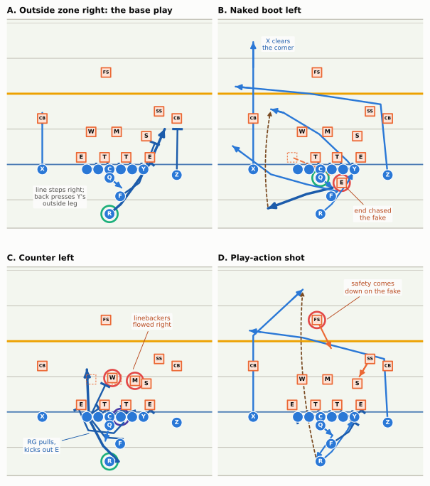
In Figure 43.3 below, cover the bottom three panels with your hand and look only at the top-left one. That is what the defense sees for the first half-second of every play in the figure: the same alignment, the same line stepping right (all but one guard, as you’ll see), the same back heading toward the tight end. A defender who waits to find out which play it is gets beaten by outside zone, because outside zone is a race to the edge. A defender who reacts at once gets beaten by one of the other three. The offense has made waiting and reacting both wrong.

How long does a defender have? Not long. A linebacker’s read happens in his first step or two, well under a second, and by the time he is sure, outside zone has already reached the edge. That is why “wait and see” is not an option for him.

LAT, WIN = (-14, 14), (-9, 20.5)
fig, axes = plt.subplots(2, 2, figsize=(6.4, 7.6))
# A. outside zone right
p = Play(offset_i(), base_43(), los=35, to_go=10)
oz_first_second(p)
go_to(p, "Y", (0.3, 5.8)); go_to(p, "FB", (3.0, 6.4), via=[(-2.6, 4.2)])
go_to(p, "RB", (5.0, 7.8), "run", via=[(-5.6, 1.6), (-2.6, 3.8), (0.0, 5.6)])
go_to(p, "Z", (5.0, 9.6)); p.route("X", [(0, 0), (8, 0)])
p.highlight("RB")
f = draw(p, ax=axes[0, 0], lateral=LAT, window=WIN)
panel_title(axes[0, 0], "A. Outside zone right: the base play")
say(f, p, -4.6, -7.0, "line steps right;\nback presses Y's\noutside leg", fontsize=6.6)
# B. naked boot left (the end is drawn where his chase has taken him; the outline shows where he started)
E_CHASE = (-2.6, 3.0)
p = Play(offset_i(), shifted(base_43(), WDE=E_CHASE), los=35, to_go=10)
oz_first_second(p, fake=True)
go_to(p, "QB", (-6.2, -7.4), "run", via=[(-4.2, -2.0)], delay=0.1)
go_to(p, "FB", (2.6, -12.4), "route", via=[(-3.8, 2.4), (-2.8, -2.0), (-1.4, -7.0)], delay=0.2)
p.route("Y", [(0, 0), (1.2, -1.0), (5.0, -5.0), (8.0, -10.0), (8.5, -11.8)])
p.route("Z", [(0, 0), (10, -1.0), (11.5, -11.0), (12.5, -21.5)])
p.route("X", [(0, 0), (18.0, 0.0)])
p.highlight("WDE", color=RED); p.highlight("QB")
p.pass_to("Y", t=4.2)
f = draw(p, ax=axes[0, 1], lateral=LAT, window=WIN)
was_here(f, p, 1.0, technique("5", -1), to=(-1.6, 2.2))
panel_title(axes[0, 1], "B. Naked boot left")
point_to(f, p, (-7.0, 7.4), E_CHASE, "end chased\nthe fake", color=style.DEFENSE_DARK)
say(f, p, 17.0, -6.0, "X clears\nthe corner", fontsize=6.4, color=style.OFFENSE_DARK)
# C. counter left (the linebackers are drawn where their flow has taken them; outlines show where they started)
p = Play(offset_i(), shifted(base_43(), MIKE=(4.4, 3.6), WILL=(4.8, 0.4)), los=35, to_go=10)
go_to(p, "LT", (0.5, -1.5)); go_to(p, "LG", (0.4, -0.4))          # play side blocks down (a step right)
go_to(p, "C", (0.3, 1.9))                                         # back block on the 3-technique
go_to(p, "RT", (0.0, 3.0)); go_to(p, "Y", (0.3, 5.8))             # the back side hinges
go_to(p, "RG", (0.5, -4.4), "pull", via=[(-1.5, 2.0), (-3.0, 0.6), (-2.6, -3.0)])
go_to(p, "FB", (3.8, -0.6), "pull", via=[(-3.8, 1.9), (-3.6, -0.6), (-0.8, -2.8)])
go_to(p, "QB", (-4.1, -0.6), "path", speed=3.0)
go_to(p, "RB", (6.0, -3.2), "run", via=[(-7.0, 1.3), (-4.8, -0.9), (-1.0, -2.9)])
p.highlight("MIKE", "WILL", color=RED); p.highlight("RG", color=PURPLE); p.highlight("RB")
f = draw(p, ax=axes[1, 0], lateral=LAT, window=WIN)
was_here(f, p, 4.6, 1.0); was_here(f, p, 4.6, -2.6)
panel_title(axes[1, 0], "C. Counter left")
point_to(f, p, (12.8, 6.0), (5.2, 3.0), "linebackers\nflowed right", color=style.DEFENSE_DARK)
point_to(f, p, (-4.8, -9.6), (-2.8, -2.0), "RG pulls,\nkicks out E", color=style.OFFENSE_DARK)
# D. play-action shot
p = Play(offset_i(), base_43(), los=35, to_go=10)
oz_first_second(p, fake=True)
go_to(p, "LT", (-1.0, -3.4), via=[(-0.5, -1.8)])                 # one zone step, then hinge back on the end
go_to(p, "QB", (-6.6, -0.6), "path", speed=3.5, delay=0.1)
go_to(p, "Y", (0.3, 5.8)); go_to(p, "FB", (-1.5, 4.8), via=[(-2.8, 4.0)])
p.route("X", [(0, 0), (11.5, 0), (18.0, -7.0)])
p.route("Z", [(0, 0), (9, -0.5), (12.0, -12.0), (13.0, -19.5)])
go_to(p, "FS", (9.0, 1.5), "path"); go_to(p, "SS", (5.0, 5.5), "path")
p.highlight("FS", color=RED)
p.pass_to("X", t=3.0)
f = draw(p, ax=axes[1, 1], lateral=LAT, window=WIN)
panel_title(axes[1, 1], "D. Play-action shot")
point_to(f, p, (17.6, 7.4), (12.6, 0.2), "safety comes\ndown on the fake", color=style.DEFENSE_DARK)
fig.tight_layout(h_pad=0.8, w_pad=0.6)
plt.show()

Figure 43.3: One formation, four plays (a Shanahan-style plate; illustrative, not a specific team’s playbook). Where to look: compare the five linemen’s first steps and R’s first step across the panels. They match, except for the right guard in C. The offense is identical before the snap in all four panels: 21 personnel, an offset I with the fullback (F) offset to the tight end’s side, the receivers in tight splits. A: outside zone right, the base play; the fullback seals the Sam inside and the back presses the tight end’s outside leg, then bounces. B: naked boot left: the same line steps and the back’s same track without the ball, and F starts on his arc before slicing back to the flat. The quarterback (thick arrow) rolls away from the backside end (red ring, drawn where his chase took him; the dashed outline is where he started), X clears the corner, and the throw (dashed brown) goes to Y crossing underneath. C: counter left: the play-side linemen block down, which is a step to the right, so their first step matches the zone step; the back takes one step right; then the right guard (purple ring) pulls back to kick out the end, and the back cuts inside that block, behind the fullback, who leads onto the Will. The linebackers (red rings) are drawn where they flowed. D: play-action shot: the same fake, seven blockers (the left tackle takes one zone step and hinges back onto the end), a post (X) and a deep crossing route (Z); the free safety (red ring) came down on the fake, so the post is open behind him. For the first half-second the defense sees the same thing four times.

Look closely and the plays aren’t perfectly identical, which matters for the arms race. On the counter the right guard pulls left instead of stepping right, a clue for a linebacker disciplined enough to read the guard instead of the back. On the naked boot nobody blocks the backside end, and that is a louder clue than it sounds: on a real outside zone somebody, the backside tackle or a tight end, cuts or cuts off that end (the block the tight end showed and then abandoned on 04-05’s naked boot), so a well-coached end’s rule is “no cut, no block: think boot.” Defenses coach to those clues (“read the guard,” “if nobody blocks you, think boot”), and offenses answer by disguising the clue: the protected boot puts a blocker back on the end, and some counters pull a tight end instead of a guard. The game never ends; it just moves to smaller details.

Why not just run the constraint play more?

Here is the puzzle that comes with every constraint play. In Perimeter Runs and Misdirection you saw that an NFL receiver’s carry (jet sweeps, end-arounds, reverses) has been worth far more on average than a running back’s, every season from 2016 to 2025. In Play-Action, Bootlegs, and Screens you saw that play-action dropbacks beat ordinary dropbacks by a wide margin, season after season. If the constraint plays are that much better, aren’t coaches leaving points on the table by calling them so rarely?

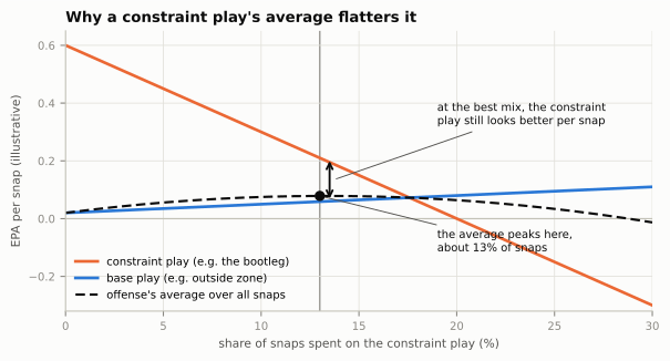
Partly, maybe. But a simple model shows why a constraint play should look better on average than the base play even when a coach is calling it exactly the right amount. Imagine the offense chooses what share of its snaps to spend on the constraint play. As that share rises, the defense sees it more on film and respects it more: it cheats less against the base play. So the constraint play gets worse the more it’s called (fewer defenders are cheating for it to punish) and the base play gets better (fewer defenders are cheating against it).

style.apply()
A_C, S_C, A_B, S_B = 0.60, 3.0, 0.02, 0.30          # constraint and base play: value = intercept + slope x share
q = np.linspace(0, 0.30, 301)
C = A_C - S_C * q
B = A_B + S_B * q
V = q * C + (1 - q) * B
qs = round(float(q[np.argmax(V)]), 2)
Cs, Bs, Vs = A_C - S_C * qs, A_B + S_B * qs, qs * (A_C - S_C * qs) + (1 - qs) * (A_B + S_B * qs)
# the worked example: move one more percentage point of snaps from the base play to the constraint play
GAIN = 0.01 * (Cs - Bs)                 # the extra constraint call is worth more than the base call it replaces
COST = qs * S_C * 0.01                  # ... but every constraint call already being made loses a little
LIFT = (1 - qs) * S_B * 0.01            # ... and every base call gains a little
fig, ax = plt.subplots(figsize=(6.4, 3.5))
ax.axhline(0, color=style.BASELINE, lw=0.9)
ax.plot(q * 100, C, color=style.SERIES[1], lw=2, label="constraint play (e.g. the bootleg)")
ax.plot(q * 100, B, color=style.SERIES[0], lw=2, label="base play (e.g. outside zone)")
ax.plot(q * 100, V, color=style.INK, lw=1.6, ls=(0, (4, 2)), label="offense's average over all snaps")
ax.plot([qs * 100], [Vs], "o", color=style.INK, ms=6, zorder=5)
ax.axvline(qs * 100, color=style.MUTED, lw=0.9, zorder=0)
ax.annotate("", (qs * 100 + 0.5, Cs), (qs * 100 + 0.5, Bs),
            arrowprops=dict(arrowstyle="<->", color=style.INK, lw=1.4))
ax.annotate("at the best mix, the constraint\nplay still looks better per snap",
            (qs * 100 + 0.7, (Cs + Bs) / 2), xytext=(19.0, 0.36), fontsize=7.5, color=style.INK,
            ha="left", va="center", arrowprops=dict(arrowstyle="-", color=style.INK_2, lw=0.7))
ax.annotate(f"the average peaks here,\nabout {qs:.0%} of snaps", (qs * 100, Vs), xytext=(19.0, -0.08),
            fontsize=7.5, color=style.INK, ha="left", va="center",
            arrowprops=dict(arrowstyle="-", color=style.INK_2, lw=0.7))
ax.set_xlabel("share of snaps spent on the constraint play (%)", fontsize=8)
ax.set_ylabel("EPA per snap (illustrative)", fontsize=8)
ax.tick_params(labelsize=7.5)
ax.set_xlim(0, 30); ax.set_ylim(-0.32, 0.65)
ax.legend(loc="lower left", bbox_to_anchor=(0.0, 0.0), fontsize=7.5, frameon=False)
ax.set_title("Why a constraint play's average flatters it", fontsize=10)
fig.tight_layout()
plt.show()

Figure 43.4: A toy model of the dose (made-up numbers chosen to make the shape visible, not estimates). As the offense calls the constraint play more often, the defense respects it more: the constraint play’s value per snap falls (orange) and the base play’s rises a little (blue). The offense’s average over all its snaps (dashed) peaks, at the dot, well before the two lines cross. At that best mix the constraint play is still worth more per snap than the base play (the bracket), yet calling it more would lower the average, because each extra call makes the defense respect it more on every snap, base plays included.

The dashed line in Figure 43.4 is what the offense actually cares about: its expected points per snap, counting every snap. It peaks at about 13% here, and at that peak the constraint play is still worth clearly more per snap than the base play. Why stop there? Work through what one more percentage point of constraint calls would do, with the toy numbers at the peak:

• The gain. One snap in a hundred switches from the base play (worth +0.06) to the constraint play (worth +0.21). That adds +0.0015 EPA per snap, averaged over all snaps.
• The cost. The defense, seeing the constraint a little more often, respects it a little more. Every constraint call the offense was already making (13% of snaps) loses about 0.03: -0.0039 per snap.
• The side benefit. A defense respecting the constraint more cheats less against the base play, so every base call gains about 0.003: +0.0026 per snap.

Add them up and the net is roughly zero. That is what “the peak” means: the value of one more call (economists say “at the margin”) has fallen to nothing, even though the average constraint call is still worth far more than the average base call. The constraint play’s average includes all the early, profitable calls; the next call only gets the margin.

So “the constraint play averages more than the base play” is not, by itself, evidence that coaches are under-using it; a well-run offense should show exactly that gap.² What the gap can’t tell you is whether a particular team is at its peak or short of it, and economists who study play-calling have argued both ways. A second reason the gap flatters constraint plays is selection: coaches call them when they see the defense leaning, so their average is built from good moments. That’s not cheating the numbers. That’s the job.

The illusion of complexity

Constraint theory says the plays must look alike. Turn that into a design principle for a whole offense and you get what coaches call the illusion of complexity: make a few plays look like many, and many plays look like one, so that the defense has to prepare for far more than the offense has to learn.³ It has two halves, and you have already seen one of them.

Many plays, one look. That’s Figure 43.3: four plays from one picture, so the picture tells the defense nothing.

One play, many looks. The other half runs the same play out of different formations, personnel groups and motions. The linemen’s assignments don’t change at all; only the costume does.

def gun_11():
    return line() + [O("QB", "QB", -5.0, 0.0, "Q"), O("RB", "RB", -5.2, -2.4, "R"), O("Y", "TE", -0.7, 4.8, "Y"),
                     O("H", "WR", -1.5, -7.0, "H"), O("X", "WR", -0.7, -10.5, "X"), O("Z", "WR", -1.5, 10.5, "Z")]


def wing_12():
    return line() + [O("QB", "QB", -1.9, 0.0, "Q"), O("RB", "RB", -7.0, 0.0, "R"), O("Y", "TE", -0.7, 4.8, "Y"),
                     O("U", "TE", -1.5, 6.4, "U"), O("X", "WR", -0.7, -9.5, "X"), O("Z", "WR", -1.5, 10.5, "Z")]


def jet_11():
    return line() + [O("QB", "QB", -1.9, 0.0, "Q"), O("RB", "RB", -7.0, 0.0, "R"), O("Y", "TE", -0.7, 4.8, "Y"),
                     O("H", "WR", -1.5, -6.5, "H"), O("X", "WR", -0.7, -10.5, "X"), O("Z", "WR", -1.5, 10.5, "Z")]


OZ_TRACK = [(-5.6, 1.6), (-2.6, 3.8), (0.0, 5.4)]
specs = [("21 personnel, offset I", offset_i(), OZ_TRACK, "defense: base 4-3, eight in the box"),
         ("11 personnel, shotgun", gun_11(), [(-4.2, 0.6), (-2.2, 3.6), (0.0, 5.4)],
          "defense: nickel, a slot corner on H"),
         ("12 personnel, wing right", wing_12(), OZ_TRACK, "defense: base, widen the edge to the wing"),
         ("11 personnel, motion away", jet_11(), OZ_TRACK, "defense: decide who travels with Z")]
fig, axes = plt.subplots(2, 2, figsize=(6.6, 4.6))
for ax, (ttl, off, via, dnote) in zip(axes.flat, specs):
    p = Play(off, [], los=35, to_go=None)
    for k in ("LT", "LG", "C", "RG", "RT"):
        p.block(k, pts=[(0.5, 2.0)])
    go_to(p, "Y", (0.3, 6.2))
    if "FB" in p.players:
        go_to(p, "FB", (2.6, 6.8), via=[(-2.6, 4.2)])
    if "U" in p.players:
        go_to(p, "U", (1.2, 8.0))
    if ttl.endswith("motion away"):
        p.motion("Z", to=(-3.6, -3.0))                 # the ball is snapped once Z has cleared the mesh
        go_to(p, "Z", (-3.8, -10.0), "path", speed=8.0)
    go_to(p, "RB", (3.4, 8.4), "run", via=via)
    p.highlight("RB")
    f = draw(p, ax=ax, lateral=(-12.5, 12.5), window=(-8.6, 4.6))
    sx, sy = _P(f, p, 0.0, 5.6)
    ax.plot([sx], [sy], marker="X", ms=7, color=style.THIRD, mec="white", mew=0.7, zorder=9)
    panel_title(ax, ttl, fontsize=8)
    ax.text(0.5, -0.04, dnote, transform=ax.transAxes, ha="center", va="top", fontsize=7.0, color=style.INK_2,
            style="italic")
fig.tight_layout(w_pad=0.5, h_pad=1.4)
plt.show()

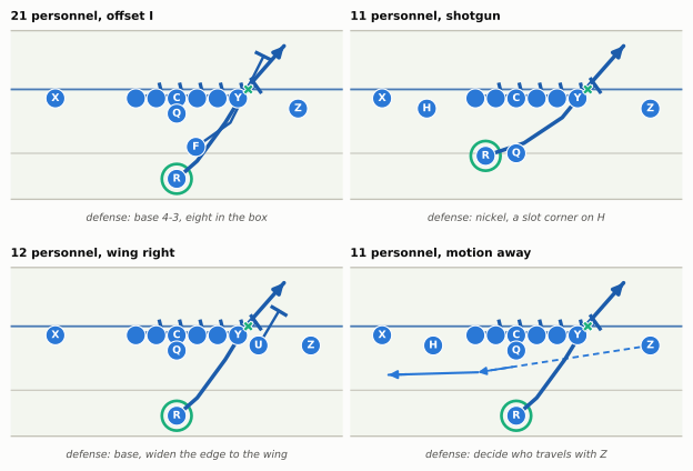
Figure 43.5: One play, four outfits: outside zone right from four different looks (illustrative). In every panel the five linemen take the same first step to the right (the short blocks ending in bars), the back aims at the same spot (the green X, just outside the tight end), and the blocking rules are identical. Only the dressing changes: two backs (21 personnel), three receivers from the shotgun (11), two tight ends with one on a wing (12), and three receivers with Z in motion across the formation away from the play, a decoy to pull defenders’ eyes and feet the wrong way. To the offense this is one play to learn. The grey note under each panel is what the defense has to change to match that look: four alignments to install and practice.

Why does this work so well? Because the burden falls unevenly. A defense doesn’t line up against a play; it lines up against a formation, with rules for who aligns where against two backs, against three receivers, against a wing, against motion. Every new look is something the defense has to install, practice and get right in a few seconds before the snap. The offense, meanwhile, practices one set of blocking rules. In Figure 43.5 the offense learned one play, and the defense had to learn four answers. Multiply by a game plan’s worth of plays and formations and the arithmetic gets lopsided fast: eight formations with three motions each is 24 pictures the defense must have an alignment for, and behind each picture could be any of a dozen core plays, so the defense prepares for close to three hundred combinations while the offense still practices a dozen plays.

The second payoff is that the outfits hide tells, the pre-snap clues you met in How to Watch a Broadcast. If an offense runs outside zone only from the offset I, the offset I is a tell. Spread the same play over four looks and every look carries several plays, so none of them gives the play away. This is a big part of why pre-snap motion has spread so fast: PFF charted a shift or motion on 63.9% of NFL plays in 2025, up from 38.4% in 2016.⁴ Motion is cheap dressing. It costs the offense almost nothing to learn and the defense a great deal to handle.

What it costs. The illusion has limits. A play still needs the right players to work: outside zone from an empty backfield is not outside zone. Every new outfit adds a little to the players’ memory load and to the chance of a busted alignment. And the outfits only stay an illusion if the plays inside them are mixed: a formation used for one play is just a tell with extra steps.

NoteFilm room: Los Angeles Rams 2018

Sean McVay’s 2018 Rams took the “one look” half of the illusion to an extreme. They used 11 personnel (one back, one tight end, three receivers) on about 93% of their plays, against a league median of about 65%, by this book’s count from nflverse data.⁵ A defense facing them could learn almost nothing from the substitution before each snap, because there was almost never a substitution: runs, play-action passes and dropbacks all came from the same eleven players, usually in a tight, condensed alignment, often with a receiver in motion. The constraint plays in 03-05’s film room (the jet sweeps that went for big gains) worked partly because they came out of the same look as everything else.

What to notice: when a team never changes personnel, stop looking at personnel and start looking at the details inside the look: the back’s depth, the receivers’ splits, which way the motion goes. That’s where a one-look offense hides, and where it sometimes leaks.

Sequencing: plays in an order

Constraint theory tells you which plays belong together. Sequencing is the order you call them in: show the defense a look, watch how it reacts, then call the play that beats that reaction. It turns a playbook into a conversation.

The idea is old. The Delaware Wing-T that you met in 03-05 was built as series football, and its coach, Harold “Tubby” Raymond, put the point bluntly: “The Wing-T is more than a formation. It is sequence football.”⁶ In the series the buck sweep comes first; the buck trap, the waggle and the counter are what the offense calls when the defense starts stopping the sweep. The mechanism is the defense’s key. Both guards pull on the buck sweep, so linebackers learn to read the guards and chase them; the rest of the series starts with the same backfield action and puts the ball where the chasing linebackers just left: inside on the trap, back the other way on the counter, and, on the waggle, a bootleg away from the sweep fake. To the linebacker reading the backfield, the constraint looks like the base play, which is the whole idea. Bill Walsh’s habit of scripting his first fifteen or so plays (the opening script that the next chapter takes apart) was partly a sequencing tool too: he planned in advance which looks to show early so he could see how the defense answered them and call the answers later.⁷

Sequencing comes in three shapes you can watch for.

1. Setting up the counter. Run the base play until the defense flows hard to it, then call the play that goes back against the flow. You don’t call the counter because the counter is good; you call it because the defense’s last three reactions say it will be.

def counter_play():
    p = Play(offset_i(labels=True), base_43(), los=35, to_go=None)
    # offense: the line's first steps look like outside zone right
    for k, e in (("LT", (0.6, -1.5)), ("LG", (0.5, -0.3)), ("C", (0.4, 1.0))):
        go_to(p, k, e, speed=1.6)
    go_to(p, "RT", (0.1, 3.6), speed=1.6); go_to(p, "Y", (0.4, 5.6), speed=1.8)
    go_to(p, "RG", (-0.5, 2.1), "block", speed=1.6)                 # the same first step as everyone else ...
    go_to(p, "RG", (0.1, -4.6), "pull", via=[(-1.5, 1.6), (-1.5, -2.8)], speed=5.5)   # ... then the pull
    go_to(p, "FB", (3.0, -1.4), "pull", via=[(-3.6, 0.2), (-3.3, -2.2), (0.2, -2.6)], speed=5.6, delay=0.35)
    go_to(p, "QB", (-2.7, 0.7), "path", speed=2.4)                 # opens to the right, like zone ...
    go_to(p, "QB", (-4.3, -0.4), "path", speed=2.6, delay=0.1)     # ... then turns back to meet the back
    go_to(p, "RB", (-7.0, 1.6), "run", speed=3.2)                  # one step with the zone flow
    go_to(p, "RB", (7.0, -3.4), "run", delay=0.15, speed=6.6, via=[(-4.6, -0.7), (-1.2, -3.0), (2.0, -3.1)])
    p.handoff("RB", t=1.17)
    # defense: the linebackers flow right with the line
    go_to(p, "MIKE", (3.9, 4.2), "path", speed=4.6); go_to(p, "WILL", (4.0, 1.6), "path", speed=4.6)
    go_to(p, "WILL", (3.0, -0.8), "path", speed=3.5, delay=0.1)
    go_to(p, "SAM", (3.0, 7.5), "path", speed=3.0)
    go_to(p, "WDE", (1.2, -4.2), "path", speed=1.0); go_to(p, "WDE", (0.6, -5.6), "path", speed=1.5, delay=0.2)
    go_to(p, "WDT", (1.0, 0.3), "path", speed=1.0); go_to(p, "SDT", (1.0, 3.2), "path", speed=1.0)
    go_to(p, "SDE", (1.2, 6.6), "path", speed=1.0)
    go_to(p, "SS", (6.0, 6.2), "path", speed=3.0); go_to(p, "FS", (10.0, -2.5), "path", speed=3.5, delay=0.6)
    return p


animation_or_strip(counter_play(), [0.3, 1.2, 1.8, 2.8],
                   ["every lineman, RG included, and R\nstep right; the linebackers start to flow",
                    "handoff going left; RG and F\npull back across",
                    "RG kicks out the end; F leads\nthrough; the Will is a step late",
                    "R is through the hole; the flow\nis on the wrong side"],
                   lateral=(-9.5, 9.5), window=(-8.5, 9.0),
                   rings=(("RB", style.THIRD), ("RG", PURPLE), ("FB", PURPLE)))

Figure 43.6: The counter, after the defense has learned to flow (simulated, BDB-format tracking; faint lines are each player’s path so far). The offense shows the outside-zone look from earlier in the game. (1) Every lineman, the right guard included, takes his first step to the right, and the back (green ring) steps right with them; the linebackers, trained by the earlier outside-zone runs, start to flow. (2) The back takes the handoff going left as the right guard and the fullback (purple rings) pull back across. (3) The guard kicks out the end on the left (the backside end of the zone fake, but the play-side end of the counter); the back cuts inside that block, the fullback leads through the hole, and the Will, who flowed, is a step late coming back. (4) The back is through the line on the side the linebackers just left.

2. Play-action off the base run. After the base run has gained yards from a look, call play-action from the same look within the next few snaps. This is the most common sequence in football, and the most watchable, because you can see it coming. Notice what 04-05 showed, though: linebackers bite on a good fake whether or not the run has been working. So coaches describe the sequence as being less about “earning” the fake with yards than about timing: a defense that has just been gashed is primed to come forward hard, its coaches have just told it to, and the offense knows that.

Is there any sign of that in the data? A little. On neutral first-and-10 snaps from 2022 to 2025, play-action passes called right after a run of 10 or more yards on the same drive averaged +0.21 EPA, against +0.11 for play-action at other times, and the gap showed up in 3 of the 4 seasons. Offenses did not call much more play-action at those moments (51% of dropbacks, against 47%), and the sample is small (581 snaps, so the gap is under two standard errors), so read it as consistent with the coaches’ timing story rather than as proof of it.⁸

3. The tendency breaker. The third shape needs two new words. A tendency is a pattern in what a team does in a given situation, formation or personnel group (running on four snaps in five from one look, throwing to the tight end on most third-and-shorts) that an opponent can find on film or in data and play against. A tendency breaker is a play called on purpose against your own tendency: a pass from the run look, a run from the empty backfield, a screen from the formation you always use for deep shots. It punishes an opponent who studied you, and it keeps the pattern honest for next week.

Put the three together and a drive starts to read like a conversation. Here is an illustrative one (not a real drive), with the defense’s side of the conversation in the last column:

Snap	Situation	The look	The call	What the defense learned
1	1st and 10, own 25	21 personnel, offset I	Outside zone right: +5	“This look means outside zone.”
3	1st and 10, own 36	Same look	Outside zone right: +7	Linebackers start flowing on the first step.
4	2nd and 3, own 43	Same look	Counter left: +11	“Don’t over-run; the back side has to fill the cutback.”
6	2nd and 4, opp. 40	Same look	Outside zone right: +5	Backside end starts crashing down the line to stop the cutback.
7	1st and 10, opp. 35	Same look	Naked boot left: +19	Too late.

(Snaps 2 and 5, a 6-yard gain each, came from other looks.) The offense ran one look five times and called three plays, and the order did the work. Snaps 1 and 3 taught the linebackers to flow, so snap 4’s counter went back against them. The counter taught the defense that the cutback side needed help, so on snap 6 the backside end stopped squeezing and started crashing down the line to take the cutback away, and that crashing end is exactly the man the naked boot on snap 7 is built to beat. Real defenses adjust like this between series, usually because a coach in the booth or on the sideline tablet tells them to; how that works in real time is in In-Game Adjustments.

CautionCommon misconception

“A balanced offense alternates run and pass.” Alternating is a pattern too, and patterns are what defenses hunt. An economic study of NFL play-calling found that teams were more likely to switch between run and pass from one play to the next than a truly unpredictable mix would be, which makes the next call easier to guess, not harder.⁹ Balance means the defense can’t tell from the look or the last play what comes next, not that the offense takes turns.

NoteFilm room: Kansas City Chiefs, Super Bowl LVII (2022 season)

Andy Reid’s offense is famous for the second half of the illusion of complexity, a huge menu of formations, shifts and motions dressing a stable core of concepts, and for sequencing that plays on what a defense did a few minutes earlier. The best-known example is the pair of fourth-quarter touchdowns in Super Bowl LVII against the Eagles, built on a return-motion play the team called “Corn Dog” (the full story is in Motion and Shifts): Kadarius Toney scored on it, and less than three minutes of game clock later Skyy Moore scored on a mirrored version to the other side. Both times the Eagles’ man defender went with the motion and the receiver was alone when he turned back.¹⁰

What to notice: the second call was the same play. Sequencing doesn’t always mean switching to a constraint. If the defense hasn’t fixed what beat it, the right next call is the same question again, and a staff that’s watching closely knows when a defense hasn’t adjusted. A year later, in Super Bowl LVIII, a renamed relative of the play produced the winning overtime touchdown: same idea, new clothes.

Tendencies and the self-scout

Every play an offense calls goes on film, and every opponent’s quality control coaches (the entry-level assistants from 01-04 who break film down into numbers) log it: down, distance, field position, personnel, formation, motion, run or pass, direction, result. From those logs come the tendencies a defense plays against on Sunday. A defense that knows an offense runs 80% of the time from a particular look can set its front, its linebackers’ keys and its safety’s depth to stop the run before the snap, and be right four times in five.

So offenses do the same thing to themselves. A self-scout is a team’s study of its own film and data, the way an opponent would study it, to find the tendencies it is giving away. Many teams do a formal one during the bye week, and the same questions come up in smaller ways all season.¹¹ The questions are the opponent’s questions: What do we do from each personnel group and formation? Which way do we run when the back is offset left? What do we do after a motion? What do we call on second-and-long after a first-down run? Where are we a coin flip, and where are we a giveaway?

What a team does with the answers is a judgment call, and there are three choices:

• Break it. Call a few tendency breakers from the giveaway look, so the next opponent’s numbers are muddier.
• Hide it. Spread the giveaway play across more outfits (the illusion of complexity again) so no single look carries it.
• Keep it as bait. Leave the tendency in place on purpose, let the opponent load up for it, and save the breaker for the moment it will hurt most: a big third down, the red zone, the playoffs.

Building a tendency table

You can run the opponent’s first question yourself. A tendency table cross-tabulates two things a defense can see before the snap (here, the offense’s personnel group and the quarterback’s alignment) and shows how often each combination produced a pass. Why the quarterback’s alignment and not the formation? Because it is the only formation information in the public data: nflverse records whether the quarterback was under center, in the shotgun or in the pistol, but not the receivers’ splits or the backfield set. A real tendency report charts far more: dozens of formation codes (2x2, 3x1, bunch, nub), the back’s offset, the motion and its direction, the hash and the field zone (“runs to the field,” “runs to the tight end,” “runs to the side the back is offset”). So whatever this table finds is a floor on what a pro staff gets from the look. To keep the situation from doing the talking (everyone throws on third-and-long), the table uses only neutral snaps: first and second down, the game reasonably close, outside the last two minutes of each half. The formal version of this filter, and expected-pass models that adjust for the situation play by play, are in Tendencies, PROE and Charting.¹²

The recipe, if you want to build one yourself (the code is under “Show the Python” on the website): load a season’s play-by-play with nflreadpy; join the participation file for personnel and the FTN charting file for the quarterback’s alignment, matching on game and play; keep the neutral first- and second-down snaps; then make a pivot table of the pass flag’s mean by personnel group and alignment, with a second pivot of counts so you can ignore cells with only a handful of snaps.

cmap = LinearSegmentedColormap.from_list("run_pass", [style.SERIES[1], style.DIVERGING[1], style.SERIES[0]])
fig, axes = plt.subplots(1, 2, figsize=(6.6, 2.9), sharey=True)
for ax, (rt, nn, ttl) in zip(axes, [(R_DET, N_DET, "Detroit Lions, 2024"), (R_NFL, N_NFL, "All 32 teams, 2024")]):
    vals = np.where(nn.values >= 15, rt.values, np.nan)
    ax.imshow(vals, cmap=cmap, vmin=0, vmax=1, aspect="auto")
    for i in range(vals.shape[0]):
        for j in range(vals.shape[1]):
            if nn.values[i, j] >= 15:
                ax.text(j, i - 0.12, f"{rt.values[i, j]:.0%}", ha="center", va="center", fontsize=9.5,
                        fontweight="bold", color=style.INK)
                ax.text(j, i + 0.24, f"n={int(nn.values[i, j]):,}", ha="center", va="center", fontsize=6.6,
                        color=style.INK_2)
            else:
                ax.add_patch(plt.Rectangle((j - 0.5, i - 0.5), 1, 1, fc=style.GRID, ec="none"))
                ax.text(j, i, "too few" if nn.values[i, j] else "none", ha="center", va="center", fontsize=6.6,
                        color=style.MUTED)
    ax.set_xticks(range(3), rt.columns, fontsize=7.6)
    ax.set_yticks(range(len(rt)), [f"{g} personnel" for g in rt.index], fontsize=7.6)
    ax.tick_params(length=0)
    for sp in ax.spines.values():
        sp.set_visible(False)
    ax.set_xticks(np.arange(-0.5, 3, 1), minor=True); ax.set_yticks(np.arange(-0.5, len(rt), 1), minor=True)
    ax.grid(False); ax.grid(which="minor", color=style.SURFACE, lw=2.5); ax.tick_params(which="minor", length=0)
    ax.set_title(ttl, fontsize=9.5)
fig.tight_layout(w_pad=1.0)
plt.show()

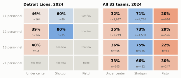
Figure 43.7: A tendency table: how often the offense passed, by personnel group (rows) and quarterback alignment (columns), neutral situations of the 2024 regular season (first and second down, win probability 20–80%, outside the last two minutes of each half). Left, the Detroit Lions in Ben Johnson’s last season as their offensive coordinator; right, all 32 teams together. Blue cells lean pass, orange cells lean run, pale cells are close to a coin flip; grey cells had fewer than 15 snaps. League-wide, the quarterback’s alignment is a loud tell: about seven passes in ten from the shotgun, three in ten from under center, two to three in ten from the pistol. The Lions were much closer to even under center. Data: nflverse play-by-play, participation (personnel) and FTN charting (alignment) via nflreadpy.

The right-hand table in Figure 43.7 is the league’s starting point, and the loudest thing in it is not personnel at all: it’s where the quarterback stands. From the shotgun, offenses passed on about seven neutral snaps in ten; from under center, about three in ten; from the pistol (the quarterback a few yards back with the back behind him), even fewer. Personnel barely moves those numbers. A defense that saw nothing but the quarterback’s feet would already be well ahead of a coin flip.

Now the Lions. In 2024, Ben Johnson’s third and final season calling Detroit’s plays, they passed on 46% of their neutral 11-personnel snaps from under center, against 32% for the league, and on about four in ten from under center with two or three tight ends. That’s a self-scouted offense: the look that screams “run” for everyone else was close to much closer to even in Detroit, because Johnson used it for play-action as readily as for runs. The shotgun was more predictable (80% passes from 12 personnel), but only on 35 snaps; Detroit lived under center, where its pictures said the least. (The empty 21-personnel cells don’t mean the Lions left the family. The modern Shanahan-tree offenses mostly hide the same one-look, many-plays idea in 11 and 12 personnel under center, with a tight end or a receiver doing the fullback’s motion and blocking jobs.)

# Change the team and season to build your own table (seasons 2022-2025 are loaded above).
rate, n = tendency_table(N, team="KC", season=2025, groups=("11", "12", "13"))
print((100 * rate).round(0).astype("Int64"))   # pass rate, %
print(n)                                        # snaps behind each cell: ignore cells with only a handful

How much does the look give away?

A table shows the pattern; the question a defensive coordinator cares about is how much it’s worth. So run the scout’s experiment honestly. For every neutral snap from 2022 to 2025, predict run or pass using only that team’s other games that season (as a scout would, from film he has already seen): if the team passed on more than half of its snaps from this personnel-and-alignment look elsewhere, guess pass. Compare that with a dumber guess that ignores the look and uses only the team’s overall lean.

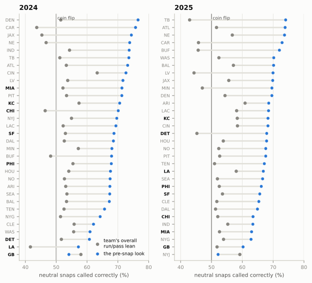
League-wide, the overall lean alone called about 53% of neutral snaps correctly, barely better than a coin. (For a team close to 50/50 overall, it can even do worse than a coin: if the team passed on 52% of snaps in its other games but ran more often in this one, every guess in this game is “pass” and most are wrong.) The look called about 67%. Two pre-snap facts, personnel and where the quarterback stands, turn a coin flip into two right guesses in three. Figure 43.8 shows how much that varied by team.

style.apply()
SHOW = {"GB", "LA", "DET", "CHI", "SF", "MIA", "PHI", "KC"}
fig, axes = plt.subplots(1, 2, figsize=(6.6, 6.0))
for ax, s in zip(axes, [2024, 2025]):
    a = ACC.loc[s].sort_values("hit_look")
    y = np.arange(len(a))
    ax.hlines(y, a["hit_team"] * 100, a["hit_look"] * 100, color=style.GRID, lw=2.0, zorder=1)
    ax.scatter(a["hit_team"] * 100, y, s=16, color=style.MUTED, zorder=2, label="team's overall\nrun/pass lean")
    ax.scatter(a["hit_look"] * 100, y, s=26, color=style.SERIES[0], zorder=3, edgecolor=style.SURFACE, lw=0.6,
               label="the pre-snap look")
    ax.set_yticks(y, a.index, fontsize=6.4)
    for lab in ax.get_yticklabels():
        if lab.get_text() in SHOW:
            lab.set_fontweight("bold"); lab.set_color(style.INK)
    ax.axvline(50, color=style.INK_2, lw=1.1, zorder=0)
    ax.text(50.4, len(a) - 0.5, "coin flip", fontsize=6.6, color=style.INK_2, ha="left", va="top")
    ax.set_xlim(38, 80); ax.set_ylim(-0.8, len(a) - 0.2)
    ax.grid(axis="y", visible=False)
    ax.set_xlabel("neutral snaps called correctly (%)", fontsize=8)
    ax.tick_params(axis="x", labelsize=7.5)
    ax.set_title(f"{s}", fontsize=10)
axes[0].legend(loc="lower right", fontsize=7, frameon=False, handletextpad=0.3)
fig.tight_layout(w_pad=1.2)
plt.show()

Figure 43.8: How much each offense’s pre-snap look gave away, 2024 and 2025 regular seasons (neutral situations). For each snap, run or pass was predicted from the team’s other games that season, using either the team’s overall run/pass lean (grey) or the pass rate of that personnel-and-alignment look (blue). Lower blue dots are harder offenses to read. In 2024 the three least predictable offenses by this measure were Green Bay, the Rams and Detroit; for Green Bay the look was no help at all. Teams named in this chapter are in bold. The dark vertical line at 50% is a coin flip. Data: nflverse play-by-play, participation and FTN charting; course calculation.

The bottom of the 2024 chart reads like a family tree. Matt LaFleur’s Packers, Sean McVay’s Rams and Johnson’s Lions were the three hardest offenses to read from the look; Green Bay’s looks were actually worse than useless, because what the Packers did from a look in one game didn’t carry over to the next. In 2025 the Packers were near the bottom again, along with the Jets (whose looks were also worse than nothing, and whose offensive coordinator that season, Tanner Engstrand, had been Johnson’s passing-game coordinator in Detroit),¹³ Mike McDaniel’s Dolphins and Johnson’s new team in Chicago. Most of the hardest offenses to read share one family of ideas: under-center outside zone, bootlegs and play-action from shared looks, the Shanahan tree and its close relatives, built around exactly the idea in Figure 43.3. At the other end, the most predictable offenses let the look call about three snaps in four for the defense.

Two cautions keep this honest. First, “predictable” is not the same as “bad”: a good offense can tell you what’s coming and do it anyway (see the Eagles below), and an unpredictable offense can still be poor at executing. This chart measures what the look gave away, not what it cost. Across the 128 team-seasons from 2022 to 2025, how well the look predicted an offense and how many points per play that offense produced were essentially unrelated (correlation -0.02); the fuller version of that question is in 13-04. Second, a team’s measure moves from year to year with its quarterback, its injuries and its coordinator, so read the shape of the chart more than any single rank.

NoteFilm room: Philadelphia Eagles 2024 — a tendency they could afford

The 2024 Eagles show the other side of the self-scout. In neutral situations they lined up in the pistol with 11 personnel 46 times and passed on 7% of them: about as loud a tell as an offense gives. They kept it anyway. Saquon Barkley ran for 2,005 yards that season behind one of the league’s best lines, and the Eagles won Super Bowl LIX.¹⁴

Knowing “run” also didn’t tell a defense which run. The Eagles’ runs carried their own built-in answers: quarterback read keeps, RPO tags, and a mix of schemes and directions, so a defense that loaded up for “run” still had to guess where.

What to notice: a tendency costs you only if the defense can do something with it. Knowing the run is coming helps a defense that can win at the line; it doesn’t help much against a line and a back that win anyway. A self-scout doesn’t break every tendency. It asks which ones the next opponent can actually exploit, and spends its tendency breakers there.

Does breaking a tendency pay?

If tendencies help defenses, then plays that go against the look should do better than plays that go with it. The data lets you test that directly. Sort every neutral snap from 2022 to 2025 by what its look said (from the team’s other games, as above): “run” if the team passed less than 45% of the time from that look, “pass” if more than 55%. Then compare what happened when the offense did what the look said, and when it didn’t.

style.apply()
fig, (a1, a2) = plt.subplots(1, 2, figsize=(6.6, 3.1), sharex=False)
rows = [("run", "Look said run"), ("pass", "Look said pass")]
y = np.arange(2)
for off, did, col, lab in ((-0.18, 1, style.SERIES[0], "offense passed"), (0.18, 0, style.SERIES[1], "offense ran")):
    m = [BRK.loc[(s, did), "mean"] for s, _ in rows]
    e = [1.96 * BRK.loc[(s, did), "se"] for s, _ in rows]
    a1.barh(y + off, m, height=0.34, color=col, label=lab, zorder=3)
    a1.errorbar(m, y + off, xerr=e, fmt="none", ecolor=style.INK_2, elinewidth=0.9, capsize=2, zorder=4)
a1.axvline(0, color=style.BASELINE, lw=0.9)
a1.set_yticks(y, [t for _, t in rows], fontsize=7.6); a1.invert_yaxis()
a1.set_xlabel("EPA per play", fontsize=8); a1.tick_params(axis="x", labelsize=7.5)
a1.grid(axis="y", visible=False); a1.set_xlim(-0.12, 0.17)
a1.legend(loc="upper center", bbox_to_anchor=(0.45, -0.30), ncol=2, fontsize=7, frameon=False)
a1.set_title("All plays", fontsize=9.5)
for off, pa, col, lab in ((-0.18, True, style.SERIES[2], "play-action"), (0.18, False, style.MUTED, "no run fake")):
    m = [PA_SPLIT.loc[(s, pa), "mean"] for s, _ in rows]
    e = [1.96 * PA_SPLIT.loc[(s, pa), "se"] for s, _ in rows]
    a2.barh(y + off, m, height=0.34, color=col, label=lab, zorder=3)
    a2.errorbar(m, y + off, xerr=e, fmt="none", ecolor=style.INK_2, elinewidth=0.9, capsize=2, zorder=4)
for i, (s, _) in enumerate(rows):
    a2.text(0.205, i, f"{PA_SHARE[s]:.0%} of these\npasses were PA", fontsize=6.6, color=style.INK_2,
            va="center", ha="left")
a2.axvline(0, color=style.BASELINE, lw=0.9)
a2.set_yticks(y, [t for _, t in rows], fontsize=7.6); a2.invert_yaxis()
a2.set_xlabel("EPA per dropback", fontsize=8); a2.tick_params(axis="x", labelsize=7.5)
a2.grid(axis="y", visible=False); a2.set_xlim(0, 0.30)
a2.legend(loc="upper center", bbox_to_anchor=(0.45, -0.30), ncol=2, fontsize=7, frameon=False)
a2.set_title("The passes, split by play-action", fontsize=9.5)
fig.tight_layout(w_pad=1.2)
plt.show()

Figure 43.9: Does going against the look pay? NFL neutral-situation snaps, 2022–2025 regular seasons. Left: expected points added (EPA) per play, by what the team’s look said from its other games (‘run’ below a 45% pass rate, ‘pass’ above 55%) and what the offense actually did. A pass from a look that usually means run was worth about twice as much as a pass from a passing look; a run from a passing look was worth no more than a run from a running look. Right: the pass rows split by play-action. Without a run fake, a pass gained the same from either kind of look; with one, both did well. Passes from run looks were mostly play-action (the share is printed on each bar), and that explains their edge. Whiskers are 95% confidence intervals; the no-fake bar for run looks rests on few snaps, so its wide whisker means ‘about the same’ is a loose statement for that bar. Data: nflverse play-by-play, participation and FTN charting; course calculation.

The left panel of Figure 43.9 is half a yes. When the look said run and the offense threw, the pass was worth +0.12 EPA on average, against +0.06 for passes from passing looks. Breaking a run tendency with a pass paid. Breaking a pass tendency with a run did not: runs were worth about the same (-0.07 and -0.07) whatever the look said.

The right panel shows why. Split the passes by whether they started with a run fake, and the difference between the looks disappears: a dropback without a fake was worth about the same from a running look as from a passing look, and a play-action pass did well from both. What made passes from run looks better is that 75% of them were play-action, against 21% from passing looks. In other words, the profitable tendency breaker in the NFL is not “surprise, it’s a pass.” It’s “surprise, it’s a pass that looks like the run you expected.” That’s constraint theory and the illusion of complexity again, showing up in the averages.

Treat this as what it is, an average over four seasons and every team, not a controlled experiment. Coaches choose when to break tendencies, and they pick good moments, so some of the gain is selection. But the asymmetry is striking, and it fits what coaches say: the run-look pass is the tendency breaker worth having.

NoteFilm room: Detroit Lions 2022–2024 — Ben Johnson’s sequencing

Ben Johnson called Detroit’s plays for three seasons, and by 2024 the Lions were the NFL’s highest-scoring offense.¹⁵ His offense was built from the Shanahan-family ingredients in this chapter, under-center runs and play-action from the same looks, plus a taste for tendency breakers. The clearest example was the sixth offensive lineman. Detroit was one of the league’s heaviest users of a “jumbo” package with an extra lineman, a look that tells most defenses “run”: league-wide, offenses passed on about 28% of neutral snaps from it in 2022–2024. Detroit passed on 33% of its 99 neutral jumbo snaps in those seasons, and 82% of those passes were play-action: a run look hiding exactly the kind of pass Figure 43.9 found profitable. The most famous jumbo snap was the extreme version of the breaker. In a December 2023 game at Dallas the Lions tried to take the lead on a two-point pass to a tackle, Taylor Decker, from a heavy look that screams run; the officials ruled that the wrong tackle had reported as eligible, and the play was wiped out.¹⁶

What to notice: watch the snap after a Lions-style big run from under center. The offense knows the defense’s coaches have just told it to come up and stop the run, and that’s the moment the same look turns into play-action. Johnson took the approach with him to Chicago as head coach in 2025, where the Bears were second in the league in play-action rate (see 04-05) and, in Figure 43.8, among the harder offenses to read.

The defense’s version: one look, several answers

Defenses play the same game from the other side. A defense has base calls too, the coverage and front it wants to be good at and calls most, and its own constraint plays: the blitz that punishes an offense for holding the ball (long play-action shots, slow-developing dropbacks, a protection that always slides the same way), and the drop that punishes a quarterback who expects a blitz and throws hot. It has tendencies the offense’s quality control coaches are hunting (does it blitz on third-and-medium? does the safety rotate toward the motion?), and it self-scouts and breaks them too.

The defensive form of the illusion of complexity is the one you met in Disguise, Rotation and Split-Field and Zone Blitzes and Simulated Pressure: show one picture before the snap and play several things after it. The offense has to decide its protection and its hot throws from the picture, so a picture that carries several defenses turns every one of those decisions into a guess.

Read Figure 43.10, below, as a constraint tree turned around. The defense’s base threat here is the Cover 0 blitz: six rushers, as many as the offense can block even with the back staying in, and nobody deep, so one missed assignment is a free rusher and the quarterback must get the ball out right now, often hot, to whoever the blitz left uncovered.

Count the threats in its top-left panel. Four linemen, two mugged linebackers and two walked-up defenders make eight possible rushers, and the offense has six blockers: five linemen and the back. It cannot block all eight, and it doesn’t try. That is the point of the look. The offense has to guess which six are coming, block those, and have a hot throw ready for anyone extra. An offense that has seen the Cover 0 version a few times learns to answer the pressure look the standard way: the quarterback identifies the Mike, the center and the back take the two mugged linebackers, and the quarterback is “hot” off any seventh rusher, throwing quick to the receiver that rusher left.

LAT, WIN = (-14.4, 14.4), (-8.8, 18.6)
fig, axes = plt.subplots(2, 2, figsize=(6.2, 5.6))
ax = axes.flat
THREATS = ("MIKE", "WILL", "NB", "SS")
p = Play(spread(), mug_look(), los=35, to_go=None)
f = draw(p, ax=ax[0], lateral=LAT, window=WIN)
threat(f, p, *THREATS)
panel_title(ax[0], "The look: eight could rush, one deep")
say(f, p, -4.6, 8.0, "who rushes?\nwho drops?", fontsize=6.8, color=style.DEFENSE_DARK)
p = Play(spread(), mug_look(), los=35, to_go=None)
for k in ("LDE", "LDT", "RDT", "RDE", "MIKE", "WILL"):
    p.rush(k)
p.man("LCB", "X"); p.man("RCB", "Z"); p.man("NB", "H"); p.man("SS", "Y")
go_to(p, "FS", (5.5, -1.6), "path"); p.man("FS", "RB")
f = draw(p, ax=ax[1], lateral=LAT, window=WIN)
panel_title(ax[1], "A. Cover 0: 6 rush, man behind")
p = Play(spread(), mug_look(), los=35, to_go=None)
for k in ("NB", "LDT", "RDT", "RDE", "MIKE"):
    p.rush(k)
p.drop("LDE", (5.0, -5.0), zone=(4, 5)); p.drop("WILL", (6.0, 0.5), zone=(4, 5)); p.drop("SS", (6.0, 8.0), zone=(4, 5))
p.drop("LCB", (14.0, -10.0), zone=(5, 7)); p.drop("FS", (14.5, 0.0), zone=(5, 7))
p.drop("RCB", (14.0, 10.0), zone=(5, 7))
p.highlight("LDE", color=PURPLE)
f = draw(p, ax=ax[2], lateral=LAT, window=WIN)
panel_title(ax[2], "B. Fire zone: 5 rush, 3 deep, 3 under")
p = Play(spread(), mug_look(), los=35, to_go=None)
for k in ("LDE", "RDE", "LDT", "MIKE"):
    p.rush(k)
p.drop("WILL", (6.0, -4.0), zone=(4, 4)); p.drop("RDT", (5.5, 3.5), zone=(4, 4))
p.drop("NB", (5.0, -9.5), zone=(4, 4)); p.drop("SS", (5.0, 9.5), zone=(4, 4))
p.drop("LCB", (14.0, -10.0), zone=(5, 7)); p.drop("FS", (14.5, 0.0), zone=(5, 7))
p.drop("RCB", (14.0, 10.0), zone=(5, 7))
p.highlight("WILL", "RDT", color=PURPLE)
f = draw(p, ax=ax[3], lateral=LAT, window=WIN)
panel_title(ax[3], "C. Simulated pressure: 4 rush, 7 drop")
fig.tight_layout(w_pad=0.5, h_pad=0.7)
plt.show()

Figure 43.10: The defense’s version: one pressure look, three answers (illustrative). Top left, the look: both linebackers mugged in the A gaps and the nickel ($) and strong safety (SS) walked up beside the ends (dashed rings: all four are blitz threats), so eight defenders could rush against six blockers, with one deep safety. A: Cover 0, six rush (the four linemen and both mugged linebackers) and everyone else plays man (dotted lines), nobody deep; the free safety comes down late to take the back. B: a fire zone, five rush, including the nickel off the edge, while the left end (purple ring) drops into a short zone: three deep, three under. C: simulated pressure, four rush (one of them the Mike), the Will and the right defensive tackle (purple rings) drop, seven cover. The protection has to be set, and the hot throw chosen, before the offense knows which one is coming.

The fire zone and the simulated pressure are the defense’s constraint plays against that answer. They drop players into the windows where the hot throws go and bring rushers from where the protection isn’t looking, so the offense’s answer to the blitz becomes the defense’s opportunity.

The same structure holds for coverage shells. A two-high shell that can rotate to Cover 3 at the snap, or a single-high look that spins back to two deep, is one picture carrying several coverages, and it constrains the quarterback’s pre-snap read the way a run-and-boot look constrains a linebacker’s first step. The defenses that lean hardest on this, such as Brian Flores’s Vikings in 06-06’s film room, are the hardest to scout, because their tendencies are built to be coin flips.

The defense also has to self-scout. A defense that always rotates the safety toward the motion, or always blitzes on third-and-6, has handed the offense a free play: motion to set the rotation, or a screen against the blitz. The cure is the same as on offense: break it, hide it, or keep it as bait for one big moment.

TipWatch for it on Sunday: call the follow-up

Pick one offense for a quarter and keep a tiny log: the look (personnel and where the quarterback stands) and the play.

Before the snap

• Is this a look you’ve already seen today? Say what it was used for last time.
• If the last play from this look was a big run, say “play-action” out loud. It’s the most common follow-up in football, usually within the next few snaps.
• Pick out the cheater: the linebacker flowing early, the backside end crashing down the line instead of squeezing, the safety creeping down. The next constraint play will be aimed at him.

After the snap

• First step: did the line go the same way as the base play? If so, watch the ball, not the line.
• Did the ball come back against the flow (counter), the quarterback roll away from it (boot), or the throw go over the safety who came down (shot)? Name the defender it punished.
• On defense: when you see a pressure look on third down, count rushers at the snap. If a mugged linebacker drops, you’ve seen the defense’s constraint play against the hot throw.

Predict the play

TipPredict the play 1: the flow and the end

p = Play(offset_i(), base_43(), los=45, to_go=6)
f = draw(p, lateral=(-13, 13), window=(-8.6, 15.5), width_in=5.4)
ghost(f, p, [(4.6, 1.0), (3.9, 2.6), (3.0, 4.2)], alpha=0.8, lw=1.6)
ghost(f, p, [(4.6, -2.6), (5.3, -0.6), (5.2, 2.8)], alpha=0.8, lw=1.6)
ghost(f, p, [(0.3, -4.5), (-0.5, -2.7)], color=style.DEFENSE_DARK, alpha=1.0, lw=1.8, zorder=9)
cx, cy = _P(f, p, 1.0, technique("5", -1))
f.ax.add_patch(Circle((float(cx), float(cy)), 1.05, fc="none", ec=RED, lw=1.7, zorder=7))
point_to(f, p, (10.8, -5.6), (5.1, -1.4), "last three runs:\nlinebackers fly right", color=style.DEFENSE_DARK)
point_to(f, p, (-4.8, -8.4), (-0.1, -3.4), "end squeezes a yard,\neyes on Q (no chase)", color=style.DEFENSE_DARK)
plt.show()

Figure 43.11: Second-and-6, second quarter. The offense is back in its favorite look: 21 personnel, offset I, tight end right. The faint dashed arrows show what the defense did on the offense’s last three outside-zone runs to the right from this look: both linebackers flew to the play side at the snap, while the backside end (ringed) now plays boot, counter, reverse: he squeezes the cutback a yard down the line but keeps his shoulders square and his eyes on the quarterback, instead of crashing down the line as he did earlier in the game.

The defense has adjusted to the outside zone and to the boot. What does the offense call, and where does the ball go?

TipAnswer

A counter to the left (or another run back against the flow), not the naked boot. Two things have changed. The linebackers are flowing even harder, which is the counter’s cue: it starts like outside zone and brings the ball back to the side they just left. And the backside end has stopped crashing. He now plays boot, counter, reverse: he squeezes a yard, keeps his eyes on the quarterback and stays at the edge. That kills the naked boot, because he is standing on the spot the quarterback would roll to, facing him.

Is the end a problem for the counter, too? Partly: a disciplined boot-counter-reverse end is also a counter defender (it’s the C in his checklist). But a squeezing end is exactly the man the pulling guard is built to kick out, and the guard comes at him from inside, with a good angle. (If he squeezes so hard that he crosses the guard’s face, the guard logs him, sealing him inside, and the back bends outside instead.) The counter still wins here because the linebackers’ over-flow is the bigger cheat, and nothing else on the tree punishes it as directly. Expect the back to take one step right, then the right guard (or the tight end, in some versions) to pull back across, kick the end out, and the fullback to lead up onto the Will, who has to stop, turn and come back.

What about the protected bootleg, branch (1) on the tree? The linebackers are flying, and it puts a blocker on the end, so it’s a reasonable second answer, and partial credit if you said it. It is worse than the counter here because of where this end is: he is waiting at the quarterback’s launch point with his eyes on the quarterback, so the boot’s lone blocker meets a defender who expects him, the quarterback has to pull up early, and the crossing routes don’t get time to come open behind the linebackers.

If you said “naked boot,” that was the right answer a few snaps ago, when the end was crashing. The tree in Figure 43.1 is a map of which defender to punish; this defense moved, so the answer moved with it. If the end starts crashing again, the naked boot comes back.

TipPredict the play 2: right after the big run

def ace_12():
    return line() + [O("QB", "QB", -1.9, 0.0, "Q"), O("RB", "RB", -7.0, 0.0, "R"), O("Y", "TE", -0.7, 4.8, "Y"),
                     O("U", "TE", -0.7, -4.8, "U"), O("X", "WR", -1.5, -11.0, "X"), O("Z", "WR", -1.5, 11.0, "Z")]


dfn = [q.moved(d=1.0, w=-5.7) if q.key == "WDE" else q for q in base_43()]
dfn = [q.moved(d=6.8, w=4.0) if q.key == "SS" else q for q in dfn]
dfn = [q.moved(w=-11.0) if q.key == "LCB" else (q.moved(w=11.0) if q.key == "RCB" else q) for q in dfn]
p = Play(ace_12(), dfn, los=72, to_go=10)
p.highlight("SS", color=RED)
f = draw(p, lateral=(-14.5, 14.5), window=(-8.6, 16.5), width_in=5.4)
say(f, p, 13.0, 4.0, "one deep", fontsize=6.8, color=style.DEFENSE_DARK)
plt.show()

Figure 43.12: First-and-10 at the opponent’s 38, early in the third quarter. Two snaps ago, from this exact look (12 personnel, under center, both tight ends attached to the line), the offense ran outside zone for 23 yards. In its neutral-situation film this season the offense has passed on about 30% of its snaps from this look. The defense has brought its strong safety (SS, ringed) down to about seven yards, and the free safety is the only deep defender.

Run or pass? If pass, what kind, and what is the defense afraid of?

TipAnswer

This is the snap for a play-action shot, and if it’s a pass it’s likely to go deep, though run is still the single most likely call. Start with the numbers: from this look the offense passes about three times in ten, so a pure tendency guess says run. That’s what the defense’s tendency report says too, and after a 23-yard run its coaches will have told it to stop the run, which is why the strong safety has come down to seven yards. That’s the lean.

Now think like the play-caller. The best time to break a tendency is when the defense is most committed to it. A play-action shot from the same look, with the same line steps and the same back’s track, attacks the one deep safety: one receiver deep down the middle to hold him, another on a deep crossing route behind the linebackers who come forward on the fake, seven or eight players blocking. Figure 43.9 is the case for it: passes from looks that usually mean run have been worth about twice as much as ordinary passes, almost entirely because they’re play-action.

A good defense knows this too, which is why many coordinators keep a safety deep for a snap or two after a big run even when the scouting report says run. That matters for the offense in two ways. If the quarterback has a check at the line and sees the defense back out of the eight-man look before the snap (the strong safety drifting back to two deep), he can check to the run, because the shot has lost its target. And if the defense disguises it and the free safety bails at the snap, the shot is covered on this play, but the offense has learned something for the next snap from this look: a defense that is guarding the deep middle has fewer men in the box, and the run is back on.

TipPredict the play 3: the third time they show it

p = Play(spread(), mug_look(), los=40, to_go=7)
f = draw(p, lateral=(-14.6, 14.6), window=(-7.6, 15.5), width_in=5.6)
threat(f, p, "MIKE", "WILL", "NB", "SS")
ghost(f, p, [(-1.0, -7.3), (1.0, -6.0), (4.2, -2.9)], color=style.OFFENSE, alpha=0.7)
point_to(f, p, (11.0, -6.0), (4.0, -3.2), "where the hot throw\nwent twice", color=style.OFFENSE_DARK)
plt.show()

Figure 43.13: Third-and-7. The defense shows the same pressure look for the third time today: both linebackers mugged in the A gaps and the nickel and strong safety walked up beside the ends (dashed rings: blitz threats), one deep safety. The first two times it was a six-man Cover 0 blitz, and both times the quarterback beat it with a quick throw to the slot receiver on his left (H), right where a blitzing Will had come from.

Six rushers again? What should the quarterback expect?

TipAnswer

Probably not six this time: expect a simulated pressure or a fire zone, with a defender dropping into H’s window. The defense’s base threat has been beaten twice in the same way: the offense now expects six, puts the center and the back on the two mugged linebackers and throws hot to the slot. That answer is exactly what the defense’s constraint plays are built to punish. The likeliest call drops one of the mugged linebackers (most likely the Will, on H’s side) straight into the short window the hot throw has been going to, and brings a rusher from somewhere the protection isn’t looking, such as the nickel off the edge (he’s walked up, so he can) or a lineman looping. Four or five rush; six or seven cover.

For the quarterback, the danger is throwing the same hot route on rhythm into a defender who is waiting for it. The better plan is to hold the ball a beat to see who actually comes, or to have a route behind the dropper. The defense can also bluff the other way and blitz six a third time, betting that the offense has adjusted already; that’s the coin flip the defense wants the quarterback to face. But after two clean hot completions, the sequencing logic points to the drop.

Takeaways

• Base plays are what an offense wants to be good at; constraint plays punish the defense for stopping them. Every constraint play is defined by the defender it punishes: find the defender who is cheating and you’ve found the play that’s coming.
• The two need each other. The base play keeps the defense leaning, the constraint plays limit the lean, and a constraint play’s average should look better than the base play’s even when it’s called the right amount, because each extra call costs a little on every other snap.
• The illusion of complexity works from both ends. One play in many outfits gives the defense more to prepare; many plays from one look gives it nothing to read. Both hide tells.
• Sequencing is the order of the conversation: the counter after the flow, play-action after the big run, the tendency breaker after a stretch of predictability. Sometimes the right follow-up is the same play again.
• Tendencies are real and measurable. In neutral situations from 2022 to 2025, personnel plus the quarterback’s alignment called about two snaps in three correctly; the hardest offenses to read came mostly from the Shanahan family of offenses. Passes from run looks paid off, mostly because they were play-action.
• Defenses play the same game: one pressure look or one shell carrying several calls, and their own self-scout.

Connections

Builds on: Perimeter Runs and Misdirection (series football and the receiver-run puzzle), Play-Action, Bootlegs, and Screens (the plays on the constraint tree), Zone Running (the base play), RPOs (constraints built into one play), How to Watch a Broadcast (tells), Disguise, Rotation and Split-Field and Zone Blitzes and Simulated Pressure (the defense’s version), and What Beats What (beaters as probabilities).

Sets up: The Game Plan: A Week Inside an NFL Building (tendency reports, the opening script and how a staff turns all of this into a call sheet); In-Game Adjustments, Tempo, and the Sideline Battle (sequencing in real time); Early Downs and Field Zones (how the situation shapes which plays are base and which are constraints); Tendencies: PROE, Personnel, Motion, and Coverage (expected-pass models and the full tendency toolkit); and the case study The Shanahan Tree, which builds an entire offense on Figure 43.3.

NoteGo deeper

Chris B. Brown’s Smart Football archive (start with the 2011 constraint-theory post in the notes) and his book The Art of Smart Football (2015) are the clearest writing on these ideas for a general reader; Harold Raymond and Ted Kempski’s The Delaware Wing-T: An Order of Football is the classic coaching text on sequence. Bill Walsh’s Finding the Winning Edge explains scripting and game-planning from the inside. For the analytics, start with this chapter’s tendency code, then 13-04; Kovash and Levitt’s paper on play-calling and game theory is a readable way into the economics of being unpredictable.

---

1. The idea is much older than the name; the name “constraint theory” was popularized by the coach and writer Chris B. Brown on his Smart Football site, for example in “Why Every Team Should Apply the Constraint Theory of Offense” (June 14, 2011), which separates an offense’s “base, core plays” from the “constraint plays” (bubble screens, play-action, bootlegs, draws, traps) that make defenders “pay for their impatience” when they cheat: https://web.archive.org/web/20110616214847/http://smartfootball.com/offense/why-every-team-should-apply-the-constraint-theory-of-offense.

2. The textbook game-theory version says something different: if both sides choose at random each snap and neither can learn from the other’s history, the offense’s best mix makes its plays equally valuable on average. Brian Burke laid out that argument for run-pass balance in “Game Theory and Run/Pass Balance,” Advanced NFL Stats, June 13, 2008: https://web.archive.org/web/20080920054748/http://www.advancednflstats.com/2008/06/game-theory-and-runpass-balance.html. The toy model here lets the defense learn how often the constraint comes from film, which is what leaves a gap in the averages. Which picture fits real play-calling better is exactly what the economists argue about.

3. The phrase is common shorthand in the Shanahan family of offenses, and its first use is not well documented. Robert Mays used it of Kyle Shanahan’s Falcons offense in “The NFL’s Newest Mastermind Eyes the Throne,” The Ringer, Jan. 30, 2017: https://www.theringer.com/2017/01/30/nfl/kyle-shanahan-atlanta-falcons-super-bowl-nfl-playoffs-4a40f26c05e2. Matt LaFleur used it on taking the Packers job in January 2019; Davante Adams said LaFleur “wants to bring in a new kind of innovative style – an illusion of complexity” (Rob Demovsky, ESPN, Jan. 28, 2019: https://www.espn.com/blog/green-bay-packers/post/_/id/46765/davante-adams-packers-offense-will-be-new-school-under-new-coach). Later profiles trace the phrase to the Washington staff (2010s) that included Kyle Shanahan, LaFleur and Sean McVay.

4. Daire Carragher, “NFL pre-snap motion usage reaches new highs across the NFL,” PFF, Feb. 23, 2026 (shift or motion on 38.4% of plays in 2016 and 63.9% in 2025): https://www.pff.com/news/nfl-pre-snap-motion-usage-reaches-new-highs-across-the-nfl. PFF’s series counts shifts as well as motion and is not comparable with FTN’s is_motion flag.

5. Course calculation from nflverse participation data, 2018 regular season, runs and passes with a recorded personnel grouping: the Rams were in 11 personnel on 92.7% of plays (about 1,040 plays); the median team was at about 65% and the next-highest team, Green Bay, at 76%.

6. Raymond’s line is quoted in Chris B. Brown, “The Making of a Modern-Day Guru,” Grantland, January 3, 2014: https://grantland.com/features/gus-malzahn-offensive-evolution/. See also Harold R. Raymond and Ted Kempski, The Delaware Wing-T: An Order of Football (Parker Publishing, 1986).

7. Bill Walsh with Brian Billick and James Peterson, Finding the Winning Edge (Sports Publishing, 1998), on scripting the opening plays; AP obituary via NFL.com (July 30, 2007), crediting Walsh with popularizing “the practice of scripting the first 15 offensive plays of a game”: https://www.nfl.com/news/hall-of-fame-coach-bill-walsh-who-won-three-super-bowls-with-th-09000d5d800879e1. Accounts of the script’s length range from 15 to about 25 plays.

8. Course calculation from nflverse play-by-play and FTN charting (is_play_action), 2022–2025 regular seasons, neutral first-and-10 dropbacks that were not the first play of a drive. “Right after a big run” means the previous snap of the same drive was a run that gained 10 or more yards. Comparing only first-and-10 snaps keeps the down and distance the same, since a big run usually ends in a fresh first down.

9. Kenneth Kovash and Steven D. Levitt, “Professionals Do Not Play Minimax: Evidence from Major League Baseball and the National Football League,” NBER Working Paper 15347 (September 2009): https://www.nber.org/papers/w15347. They report negative serial correlation in NFL run-pass choices (teams switch more than an unpredictable mix would: other things equal, a team that has just passed is about 10 percentage points less likely to pass next) and argue that teams passed too rarely in the seasons studied (2001–2005); summary in the NBER Digest, October 2009: https://www.nber.org/digest/oct09/w15347.html.

10. “Corn Dog (American football),” Wikipedia: https://en.wikipedia.org/wiki/Corn_Dog_(American_football) (Toney 5-yard touchdown at 12:04 and Moore 4-yard touchdown at 9:22 of the fourth quarter; the Super Bowl LVIII version, renamed “Tom and Jerry,” for Mecole Hardman’s walk-off touchdown); Super Bowl LVII result, Kansas City 38, Philadelphia 35 (Feb. 12, 2023): https://en.wikipedia.org/wiki/Super_Bowl_LVII.

11. For example, Titans coach Mike Munchak on his staff’s 2012 bye week: “see what our tendencies are … how other teams look at us as an offense, defense, special teams” (“Titans Coaches Using Bye to Scout Own Team,” TennesseeTitans.com, Nov. 13, 2012: https://www.tennesseetitans.com/news/titans-coaches-using-bye-to-scout-own-team-8831526); and Matt LaFleur’s 2019 Packers, whose offensive and defensive staffs studied each other’s side of the ball over the bye for “a different perspective of how opponents would attack one side of the ball, where we think there could be holes or potential holes” (Mike Spofford, “Packers taking hard look at themselves over the bye,” Packers.com, Nov. 11, 2019: https://www.packers.com/news/packers-taking-hard-look-at-themselves-over-the-bye).

12. Method for every chart in this section: nflverse play-by-play (load_pbp) joined to participation (load_participation, for personnel) and FTN charting (load_ftn_charting, for the quarterback’s alignment: qb_location U, S or P), regular seasons 2022–2025. Neutral = first or second down, win probability 0.20–0.80, more than two minutes left in the half. Personnel = backs (RB + FB) then tight ends. “Pass” = nflverse’s pass flag, so sacks and scrambles count as passes. The predictions use only the team’s other games in the same season (a look needed at least eight snaps elsewhere; otherwise the team’s overall rate was used). Participation data for 2023 onward comes from FTN and earlier seasons from NGS, so personnel is coded differently across the 2022/2023 break; the backs-and-tight-ends count used here is unaffected. A sixth offensive lineman is not counted as a tight end here, so “jumbo” snaps fall into 11 or 12 personnel; that is about 3% of neutral snaps league-wide in 2024 and about 7% of Detroit’s (28 of 418, mostly coded 12), too few to move the tables. The Lions film room counts those jumbo snaps separately (six or more offensive linemen in the participation data). RPOs are coded by what happened, so an RPO that ended in a handoff is a run; that pushes RPO-heavy offenses’ looks toward whichever answer they chose after the snap, and is one more reason to read the hit rates as rough.

13. Associated Press, “Jets hire Tanner Engstrand as offensive coordinator and Chris Banjo as special teams coordinator” (Feb. 1, 2025), which describes Engstrand as the Lions’ passing game coordinator: https://www.news4jax.com/sports/2025/02/01/jets-hire-tanner-engstrand-as-offensive-coordinator-and-chris-banjo-as-special-teams-coordinator/. The Jets’ offensive coordinator for 2026 is Frank Reich (course fact sheet).

14. Pro Football Reference, Saquon Barkley (2,005 rushing yards in 2024): https://www.pro-football-reference.com/players/B/BarkSa00.htm; Super Bowl LIX, Feb. 9, 2025: Philadelphia 40, Kansas City 22 (course fact sheet). The pistol figures are a course calculation (method in the note on neutral situations).

15. Detroit went 15–2 in 2024 and led the NFL with 564 points (33.2 a game): Pro Football Reference, 2024 Detroit Lions: https://www.pro-football-reference.com/teams/det/2024.htm. Johnson was Detroit’s offensive coordinator from 2022 to 2024 and became the Bears’ head coach in 2025 (course fact sheet). Points and record also check against nflverse schedules (564 points in 17 games; Buffalo next with 525).

16. Detroit at Dallas, Dec. 30, 2023 (Week 17), Cowboys 20, Lions 19. After the game referee Brad Allen said in a pool report that No. 70 (Dan Skipper), not No. 68 (Decker), had reported as eligible; see “2023 Detroit Lions season,” Wikipedia: https://en.wikipedia.org/wiki/2023_Detroit_Lions_season, and Associated Press, “Lions take issue with officials after potential winning 2-point pass is negated by penalty” (Dec. 31, 2023): https://www.ksat.com/sports/2023/12/31/lions-take-issue-with-officials-after-potential-winning-2-point-pass-is-negated-by-penalty/. Detroit’s sixth-lineman share (9.8% of runs and passes in 2022, second to Cleveland) is from Personnel Groupings.